How the certificates work, on a pendulum
The ideas behind the lift’s certificates, each shown first on a pendulum pumped up to its upright and then on the lift itself.
Who this page is for. Readers who know some dynamics and control but not set-based verification. It condenses the explanatory chapter of the project’s technical report. Every pendulum number and figure on this page comes from two short scripts that call the certifier’s own set operations, so the pendulum runs the same code as the lift. Each idea is shown on the pendulum first; a shaded box then says what the same idea is on the lift.
The lift, in one paragraph. A block rests on the floor in front of a step. A disk, too weak to carry the block, must get it onto the step. It does so indirectly: it pushes the block against the step’s corner so that the block tilts about its floor corner (the pivot), then pushes it up and over so that it lands on the step in motion (the landing), and finally slides it into place. The plan is a chain of pieces, and each piece comes with a feedback law and a certificate. See Certified funnels for the chain.
1. The question: what does it mean to certify a motion?
A test runs one starting state and watches what happens. A certificate is a statement about every state in a set: for every starting state in the piece’s entry set, every disk friction in the declared band and every disturbance in a measured set, the motion stays inside a tube, the contacts behave as planned, and the motion leaves through an exit set that lies inside the next piece’s entry set. Pieces then chain by set containment.
Why a simulator alone cannot do this. A simulator runs one state at a time, and a set holds infinitely many. Between two samples the motion can change in kind: two landings a millimetre apart can end one with the block sticking on the step corner and landing, the other with the block slipping back to the floor. details: issue #63 No number of samples rules out a third, unsampled outcome. So the certificates push whole sets of states through a model whose step can be bounded, and the simulator is used for what it does well: measuring how far the model is from it (Section 9).
2. The running example
A rigid pendulum of length \(l = 1\) m swings under gravity with a torque \(u\) (per unit inertia), \(\theta = 0\) hanging down: \[ \ddot\theta = -\tfrac{g}{l}\sin\theta + u, \qquad |u| \le u_{\max} = 4\ \text{rad/s}^2 . \] Its energy per unit inertia is \(E = \tfrac12\dot\theta^2 - \tfrac{g}{l}\cos\theta\). Without input the energy is constant and the state moves along a level curve of \(E\). One level is special: \(E^* = g/l\) passes through the upright \(\theta = \pm\pi\) with zero speed. The orbit on it, the homoclinic orbit, approaches the upright and takes infinitely long to get there. On it the speed is a function of the angle, \[ \dot\theta = \pm\,\omega(\theta), \qquad \omega(\theta) = 2\sqrt{g/l}\,\cos(\theta/2), \] 6.26 rad/s at the bottom and zero at the top.
The law. Åström and Furuta’s energy shaping [1] pumps energy in until the state reaches that orbit: \[ u = \operatorname{sat}\big(k\,(E^* - E)\,\dot\theta\big), \qquad k = 0.1, \] where \(\operatorname{sat}\) clips to \(\pm u_{\max}\). Physically: push along the motion while the energy is too low, against it while it is too high. Since \(\dot E = \dot\theta\,u\), the unsaturated law gives \(\dot E = k\,(E^* - E)\,\dot\theta^2\), which moves \(E\) toward \(E^*\) and stops only when the pendulum is at rest. From near the bottom the swing grows for 5 to 10 s until the orbit is reached.
The step. The model is stepped the way the simulator (MuJoCo) steps: semi-implicit Euler with \(h = 10\) ms, velocity first, then position with the new velocity: \[ \dot\theta^+ = \dot\theta + h\big(-\tfrac{g}{l}\sin\theta + u\big), \qquad \theta^+ = \theta + h\,\dot\theta^+ . \] The certificate is a statement about this map, call it \(F\), just as the lift’s certificates are statements about its 10 ms rigid step.
| Concept | Pendulum | The lift (the pivot) |
|---|---|---|
| model that is propagated | rigid pendulum, semi-implicit Euler | reduced rigid contact model, same step |
| target motion | homoclinic orbit \(\dot\theta = \omega(\theta)\) | a designed orbit \(\dot\theta = \omega(\theta)\) |
| progress variable (where along the motion) | \(\theta\), while \(\dot\theta > 0\) | the block’s tilt \(\theta\) |
| transverse coordinate (distance from the target) | \(E - E^*\), or \(\eta = \dot\theta - \omega(\theta)\) | \(\eta = \dot\theta - \omega(\theta)\), and the disk’s place on the face |
| law | energy shaping | a push \(c = c^* + K_\eta\,\eta + K_k\,(k - k^*)\) |
| modes | saturated or not | each contact sticking, sliding or open |
| what the model leaves out | bearing friction, a lagging motor | the simulator’s soft contacts, penetration, solver |
On the lift: the reduced model. The block and the disk have five coordinates (the block’s position and tilt, the disk’s position). On one piece of the plan, which contacts are closed is given by the plan, and so is each contact’s mode: a contact slides only where the geometry forces it to, and in that direction; otherwise it sticks. Each closed contact pins one combination of coordinates (its gap stays zero), and each sticking contact pins another (its material point does not slide). On the pivot these constraints leave the block a single free coordinate, its tilt. The rigid-body equations along that one-coordinate family are three linear equations in three unknowns (the tilt’s acceleration and the two normal forces), solved in closed form; a unique solution in this mode exists exactly when their determinant is nonzero, and that is checked. Like “a rigid pendulum with a torque”, this is a deliberate reduction: rigid bodies, one fixed mode per piece, a disk that does not roll. Everything left out becomes a disturbance that is measured (Section 9).
3. One step: pushing a set through the map
A certificate speaks about every state in a set, so the basic operation is: given a set of states, compute a set that surely contains all their images after one step.
Zonotopes, in plain words. A zonotope is a centre \(c\) plus a few arrows (the generators, the columns of a matrix \(G\)), each scaled by its own weight between \(-1\) and \(1\): \[ Z = \{\, c + G\xi \;:\; \xi \in [-1, 1]^m \,\}. \] With two arrows in the plane it is a parallelogram; with more, a centrally symmetric polygon. A box is the special case with the arrows along the axes. A linear map takes a zonotope to a zonotope exactly: the centre moves and the arrows are stretched and turned.
The straight-line guess. Near the centre the step is almost linear: \(F(z) \approx F(c) + J_c\,(z - c)\), with \(J_c\) the Jacobian at the centre. Applied to the zonotope, this guess gives another zonotope, \(F(c) + J_c G\,\xi\). It is exact at the centre and gets worse away from it.
What \(R\) is. \(R\) is the error margin of the straight-line guess: a number per coordinate that bounds how far the true image can be from the guess, anywhere in the set. It is
(how much the slope anywhere in the set can differ from the slope at the centre) \(\times\) (how far the set reaches from the centre).
The enclosure is “the straight-line image, plus or minus \(R\)”, and \([-R, R]\) is appended as new generators, so that later steps turn it along with the rest instead of boxing it.
The formula. The slope “anywhere in the set” is an interval Jacobian \([J]\): a matrix of intervals, each containing that partial derivative at every state of the set’s bounding box. It is computed by interval arithmetic on the step’s own code, with outward rounding [2]. It is a slope bound for this set, never a global Lipschitz constant. Then \[ F(Z) \subseteq F(c) + J_c G\,\xi \;\oplus\; [-R, R], \qquad R = \big|[J] - J_c\big|\,\big(|G|\,\mathbf 1\big) + \text{rounding}. \] Why this is sound: by the mean value theorem, row by row, \(F_i(z) - F_i(c) = \nabla F_i(\zeta)\cdot(z - c)\) for some point \(\zeta\) between \(c\) and \(z\). That point is never computed. It lies in the bounding box, and \([J]\) covers the Jacobian at every point of the box, so whatever \(\zeta\) is, its slope differs from the centre’s by at most a row of \(|[J] - J_c|\). Only computable pieces enter: \(F(c)\) and \(J_c\) (one evaluation each), \([J]\) and \(G\). The pessimism comes from using the box’s worst slope in place of the unknown \(\zeta\). (A one-line warm-up: for \(f(x) = x^2\) on \([1, 3]\), \(f(c) = 4\), \(J_c = 4\), \([J] = [2, 6]\), so \(R = 2\) and the enclosure is \([-2, 10]\), which contains the true image \([1, 9]\).)
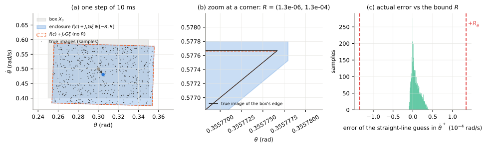
On the pendulum. Take the box \(\theta \in [0.25, 0.35]\) rad, \(\dot\theta \in [0.4, 0.6]\) rad/s near the bottom: \(c = (0.3, 0.5)\), \(G = \operatorname{diag}(0.05, 0.1)\). Over this box the law’s argument stays in \([0.75, 1.15]\), well inside \(\pm 4\), so the step is the smooth, unsaturated map (Section 6 says how that is proved). The pieces:
- the centre’s image \(F(c) = (0.3048, 0.4805)\);
- the Jacobian at the centre and the interval Jacobian over the box, \[ J_c = \begin{bmatrix} 0.99905 & 0.010188 \\ -0.09517 & 1.01881 \end{bmatrix}, \quad [J] = \begin{bmatrix} [0.99903,\ 0.99907] & [0.010185,\ 0.010191] \\ [-0.09707,\ -0.09312] & [1.01849,\ 1.01908] \end{bmatrix}; \]
- the slope spread \(|[J] - J_c|\) times the reach \(|G|\mathbf 1 = (0.05, 0.1)\) gives \(R = (1.3\cdot 10^{-6},\ 1.3\cdot 10^{-4})\);
- the new generators \(J_c G\): the box is sheared, because the angle picks up \(h\dot\theta\) and the speed picks up gravity’s pull, plus the two remainder generators \(\operatorname{diag}(R)\).
The enclosure contains the true images of all 4,004 sampled states, corners included. The largest actual error of the straight-line guess is \(0.31\,R\): \(R\) is a bound, safe and pessimistic, not the error itself.
On the lift. Within one contact mode, one 10 ms step of the reduced model running its law is an explicit smooth formula, and each set is pushed through it the same way. The step’s code is evaluated in affine arithmetic [3], with a rigorous remainder for each elementary operation and outward rounding; an operation without such a rule raises an error instead of passing silently. A piece starts from one entry set: a box of states written as a zonotope (six coordinates on the landing).
4. Many steps: rotation, growth and reduction
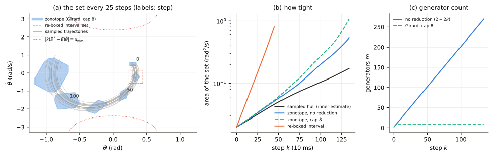
Repeat: each step maps the current zonotope and appends two remainder generators. Figure 2 follows the box above for 134 steps (1.34 s), while the pendulum swings from \(\theta = 0.3\) to \(-1\) rad and back. The set stretches, because the pumping amplifies small differences in amplitude, and it turns with the swing. At step 134 the run stops: the bound on the input over the set reaches the motor’s limit (\(4.11 > u_{\max} = 4\)), so the unsaturated mode can no longer be proved, although the sampled states themselves use at most 1.75. The set is still far from the switching curve; it is the enclosure’s over-approximation that reaches the limit.
- Generators pile up. Without reduction the count is \(2 + 2k\): 270 generators at step 134.
- Girard’s reduction [4] keeps the generators that boxing would hurt most and replaces the rest by a small box. This is sound (the result still contains the set) and costs some tightness: with at most 8 generators the area at step 134 is 1.07, against 0.53 unreduced and 0.17 for the sampled states’ convex hull (an inner estimate of the true set).
- Boxes fail where zonotopes don’t. Replacing the set by its bounding box after every step (plain interval propagation) loses so much that at step 25 its area is 0.150 against the zonotope’s 0.034, and at step 46 it can no longer prove the mode at all. A box cannot represent a tilted set, so each step re-wraps a tilted set in a larger upright box: the wrapping effect.
On the lift. The landing’s impact window, a handful of 10 ms steps in which the block hits the step, is where boxes fail and zonotopes succeed. It is certified on all 16,384 units of its six-dimensional entry set: 310,372 certified pieces and none left uncertified. Re-boxing after every step would need about \(2^{36}\) pieces. See Background: zonotope propagation.
5. Splitting: why smaller sets are much tighter
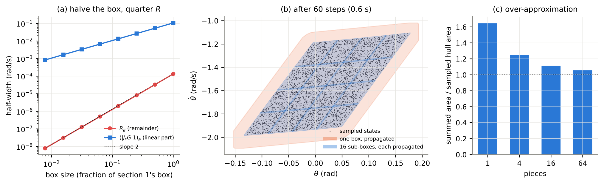
\(R\) is (slope spread) \(\times\) (reach), and both factors shrink in proportion to the set’s size. So \(R\) grows with the square of the size: halving the box quarters \(R\) while only halving the straight-line part. On the pendulum the fitted slope of \(\log R\) against \(\log(\text{size})\) is 2.01 over seven halvings, from \(1.3\cdot 10^{-4}\) down to \(7.8\cdot 10^{-9}\) rad/s.
So cutting a box into pieces and propagating each piece separately gives a tighter union. From a box 1.5 times the size of the one above, after 60 steps, the pieces’ summed area over the sampled hull’s area is 1.65 for one piece, 1.25 for 4, 1.11 for 16 and 1.06 for 64. The price is the number of pieces, which grows exponentially with the dimension. Splitting where needed, and only there, is branch and prune.
On the lift. The landing certifies with pieces between \(2^{-4}\) and \(2^{-8}\) of the entry box per coordinate, chosen by branch and prune. Splitting every coordinate to the finest size everywhere would need about \(10^{10}\) pieces. See Background: techniques that made the chain certify.
6. Modes: exclusion, not bounding
The enclosure of Section 3 needs a smooth map. A step that switches mode inside the set (the input saturates for some states and not others; a contact sticks for some and slides for others) is not smooth there. The certifier never bounds across a switch; it excludes it. Over the whole set it proves that one mode’s conditions hold, so nothing discontinuous happens inside the certified set. Where that cannot be shown, it splits the set or refuses it.
On the pendulum, saturation is the mode switch. Before each step the law’s argument \(k(E^* - E)\dot\theta\) is bounded over the current set (the same enclosure, applied to that one scalar):
- its whole range inside \((-u_{\max}, u_{\max})\): the step is the unsaturated map;
- its whole range above \(u_{\max}\) (or below \(-u_{\max}\)): the step is the saturated map \(u = \pm u_{\max}\), also smooth;
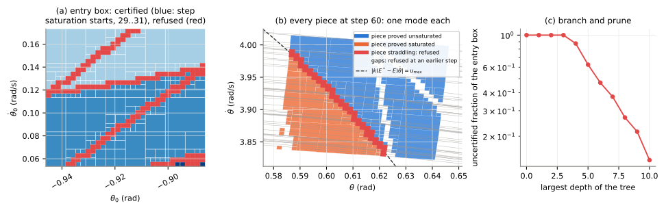
- otherwise the set straddles the switching curve: refused, and the entry box is split and each piece tried again, down to a largest depth.
Figure 5 takes an entry box 30 steps before the swing reaches saturation and an 80-step horizon in which the pendulum enters and leaves the saturated region. No piece certifies at depths 0 to 3: every one straddles at some step. At depth 10, 167 pieces certify, each with a single mode at every step (saturation starting at step 29, 30 or 31), and 140 are refused. The certified fraction of the entry box grows with depth: 0.13 at depth 4, 0.53 at 6, 0.73 at 8, 0.86 at 10. The refused pieces form thin bands, the entry states whose motion lands right on the switching curve at some step. They shrink with depth but never vanish, because those states really do switch “inside” any set around them.
On the lift, the modes are the contacts’, and the conditions are physical. Over each set the certificate proves: every closed contact presses with at least a minimum normal force; every sticking contact’s force lies strictly inside its friction cone (the disk’s at the low end, 0.3, of its friction band); every sliding contact slips in its planned direction and no faster than a measured bound; and the mode’s determinant is nonzero. The other modes are excluded too: on the pivot, all 15 alternatives (each environment contact sliding or opening, the disk sticking, sliding either way or opening) are excluded on every one of its 3,521 bands. At the landing every unplanned contact class is excluded at every step of the impact window. See Background: the contact-class solve.
7. The tube around an orbit
The progress variable. On the homoclinic orbit with \(\dot\theta > 0\) the angle keeps increasing, so \(\theta\) itself can say “where along the swing” we are, without a clock. The target becomes a function of \(\theta\), \(\dot\theta = \omega(\theta)\), and the distance from it is the transverse coordinate \(\eta = \dot\theta - \omega(\theta)\). On the energy level the two measures are tied: \(E - E^* = \omega\eta + \eta^2/2\). (During the pumping, \(\theta\) swings back and forth and indexes nothing; so the tube below covers one swing near the orbit, from \(\theta_0 = -2.6\) to \(\theta_1 = 2.6\) rad, where \(\dot\theta\) stays above 1.3 rad/s.)
The law contracts the transverse coordinate per unit of progress. Dividing \(\dot E\) by \(\dot\theta\), \[ \frac{d(E - E^*)}{d\theta} = -k\,\dot\theta\,(E - E^*), \] so over one swing the energy error shrinks by a factor of about 0.09.
The tube, indexed by progress. Cut \([\theta_0, \theta_1]\) into 473 narrow bands. Each band holds an interval of \(\eta\). The image of each band under one step is enclosed as in Section 3 and added to the bands it reaches, all of them later bands, because \(\theta\) advances by more than a band’s width per step (so one forward pass computes the tube). On every band two things are checked: the unsaturated mode (smallest margin 3.67 of the 4 rad/s² available) and the advance (smallest margin 0.0033 rad). From \(\eta \in [-0.3, 0.3]\) rad/s (an energy error of \(\pm 0.61\)), the tube narrows to \([-0.026, 0.061]\) at the bottom and leaves through \([-0.156, 0.041]\). All 200 sampled trajectories stay inside it.
Indexed by time, the same set spreads along the orbit. Propagated as sets at fixed times, the states that started slightly faster run ahead; the set stretches along the orbit (its \(\theta\) spread reaches 1.17 rad), and because the orbit is curved, the convex set’s \(\eta\) range blows up to about \(\pm 4\) rad/s near the top, where the mode can no longer be proved. Nothing pulls the states together along the path, so a certificate that does not depend on a clock should not carry that direction as a coordinate. That is why the lift’s tubes are indexed by a progress variable.
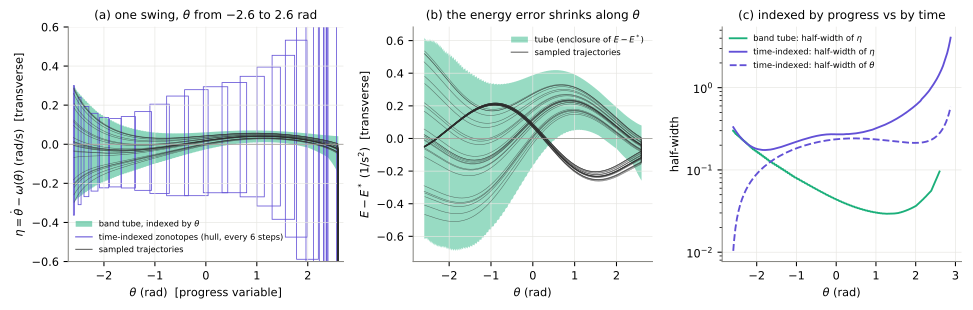
On the lift. On the pivot the progress variable is the block’s tilt, and the certificate checks that the tilt keeps increasing at a positive minimum rate over the whole tube. The target orbit is not given by physics: it is designed, as a tilt rate \(\omega(\theta)\) chosen so that each sliding contact slips no faster than a rate measured in the simulator, with the contact nearest its limit dominating (like resistors in parallel). The law reads the tilt, not a clock: \(c = c^*(\theta) + K_\eta(\theta)\,\eta + K_k(\theta)\,(k - k^*)\), a push along a fixed direction. Here \(c^*\) is the push that follows the orbit exactly, and the gains are chosen from a linearization so that, to first order, \(\dot\eta = -\lambda\eta\). The linearization is for design only: the tube is computed on the full nonlinear model running this exact law, so a linearization error can make the tube loose but never the certificate false. The pivot’s tube has 3,521 bands and a transverse half-width of 0.91°/s in tilt rate. This is maneuver regulation with transverse coordinates [5], [6], [7], and the tubes compose by “exit set inside the next entry set” [8]. See Background: certified funnels and composition.
8. Sampling versus sets
Sample 1000 starting states uniformly in the box \(\theta \in [-0.1, 0.1]\), \(\dot\theta \in [-0.2, 0.2]\) and run the closed loop for 12 s. All 1000 reach the orbit (\(|E - E^*| \le 0.25\)), in 5.3 to 9.9 s. From 1000 successes out of 1000, the Clopper–Pearson bound [9] says: with 95% confidence, at most 0.3% of the box fails. That statement is true.
But the box contains the equilibrium \((0, 0)\), where \(u = 0\) and the pendulum never moves, and states near it take arbitrarily long to get going. A fine grid gives the true failing fraction for a time budget \(T\): 0.056 at 8 s, \(1.2\cdot 10^{-3}\) at 10 s, \(2.4\cdot 10^{-5}\) at 12 s. It is never zero, and 1000 samples never see it. The statement “every state of this box reaches the orbit within 12 s” is false, so no certificate of it can exist, and the set computation agrees: no enclosure of a set containing the equilibrium can prove progress there.
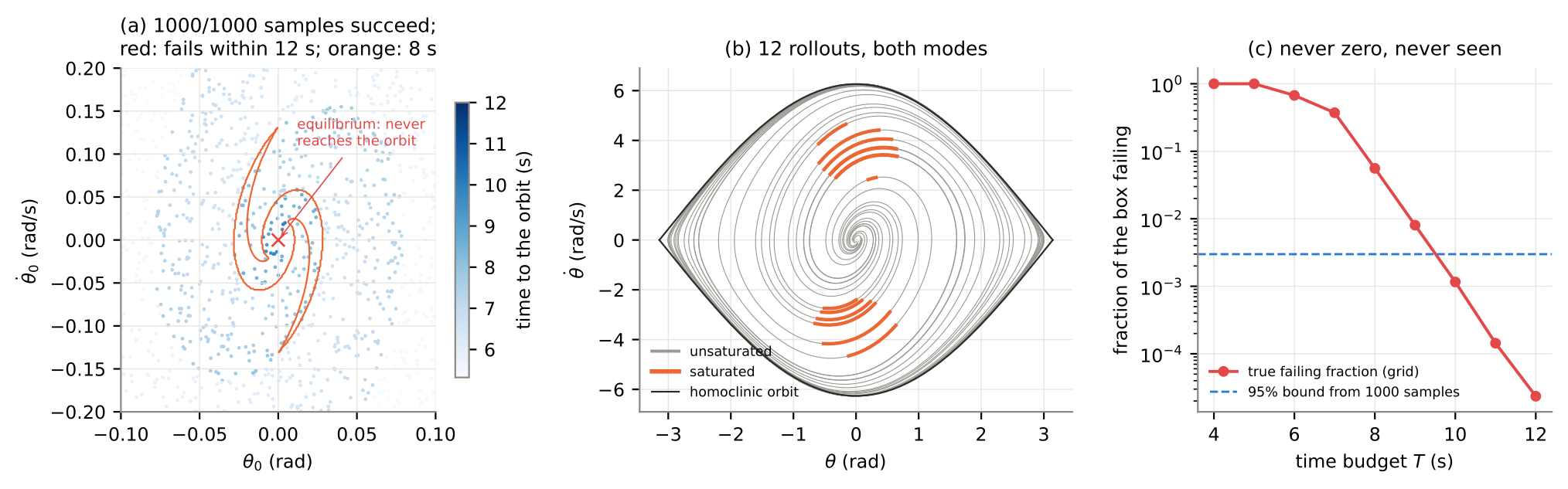
Rollouts give a probabilistic certificate: a statement about random starts drawn from a stated distribution [10], [11]. That is the right tool when the question is a probability, and the wrong tool when the question is “every state of this set”, which is what chaining pieces needs.
On the lift. The simulator’s step (MJX, the JAX version of MuJoCo) has an iterative soft-contact solver and branches on contact detection, so there is no usable enclosure of a set through it. The design therefore proves set statements on a model it can bound and uses statistics only for the model–simulator gap. What this buys:
- Every state, not random ones. A junction certifies that a whole exit set lies inside the next entry set. A statement about random starts does not chain: the next piece’s starts are wherever this piece’s motions end, not distributed like its samples.
- Composition does not degrade. Sixteen junctions at a failure probability \(\epsilon\) each could cost \(16\epsilon\); set containment composes exactly.
- The statistics are small, rich and reusable. One quantity, the one-step residual (next section), which every simulated step samples and which carries over to other entry sets, laws and pieces with the same contacts.
- It explains itself. Each condition comes with its margin, so a failure says which constraint binds.
The costs: conservative bounds, expensive splitting, the need for a rigid model close to the simulator, and a statistical residual. Simulation-based funnels exist too [12]; theirs are probabilistic, these are proved on the model.
9. The bridge to the simulator: the residual \(\mathcal W\)
Neither the pendulum’s model nor the lift’s rigid model is the system that actually runs. The certificate covers the running system without propagating it, in four steps:
- Write the true step in terms of the model’s step: \(x^+_{\text{true}} = F(x) + w\). The one-step residual \(w\) collects everything the model leaves out. In the simulator: penetration, compliance, solver tolerance.
- Measure \(w\); do not propagate it. Along many rollouts of the true system, compare each true step with the model’s step from the same state: one model evaluation per step, no sets. A 95/95 bound (covering 95% of rollouts with 95% confidence) gives the disturbance set \(\mathcal W\).
- Propagate the model with \(\mathcal W\) over sets: \(X_{k+1} \supseteq F(X_k) \oplus \mathcal W\), an enclosure plus a Minkowski sum per step. This is the certified tube: it contains every motion of “model plus any disturbance in \(\mathcal W\) at every step”.
- Coverage. A true motion is a model motion driven by its own residuals. If each residual lies in \(\mathcal W\), the true motion stays in the tube.
So the guarantee has two layers:
- Proved: if the residuals lie in \(\mathcal W\), the true system stays in the tube.
- Measured: the residuals lie in \(\mathcal W\), at 95/95; and held-out rollouts are checked to stay inside.
On the pendulum. The “true” pendulum adds what the model leaves out: bearing friction (\(b = 0.01\) 1/s) and a motor that delivers the commanded torque through a 30 ms lag. Each of 600 calibration rollouts starts near the orbit, and every step gives a residual (76,944 steps). For each rollout take the largest \(|w|\) per coordinate; over the 600 rollouts, the 580th smallest bounds 95% of rollouts at 95% confidence (Wilks’ order statistic [13]). That gives \(\mathcal W = [\pm 6.1\cdot 10^{-6}\ \text{rad}] \times [\pm 6.1\cdot 10^{-4}\ \text{rad/s}]\).
- The tube of Section 7 with \(\mathcal W\) added at every step still certifies.
- Of 600 new rollouts, all 600 stay in the tube computed with \(\mathcal W\), against 225 in the tube of the ideal model alone: the friction’s steady drag pulls the rest out.
- In 584 of the 600, every residual lies in \(\mathcal W\); in the other 16, some residual is just outside. Those 16 still stay in the tube, because the tube is a worst case over \(\mathcal W\) at every step, which a real sequence of residuals never attains.
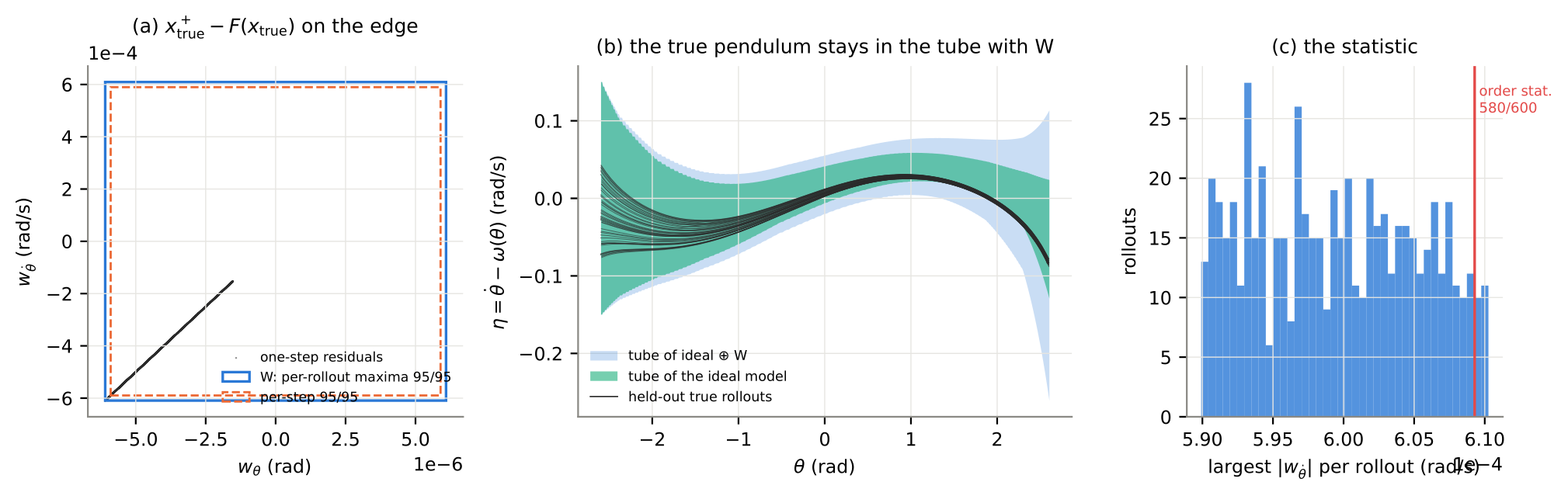
On the lift. On the pivot the residual is an extra term on the tilt acceleration, bounded at 0.556 rad/s² from 4,000 simulator rollouts, plus a measured creep bound of 0.116 mm. Of the held-out rollouts that entered the entry set, 971 of 971 (disk friction 0.5) and 967 of 968 (friction 0.3) stayed in the tube; the tube without the measured residual and creep contained none of them entirely. On the wide transport piece, 731 of 731 held-out rollouts that entered the funnel stayed inside; 49 of 780 did not enter, because a quantity the plan holds fixed while a contact sticks (a constant of motion) creeps on the way in, and all 49 still completed the transport. details: issue #77 The guarantee is therefore conditional and about the simulator; about hardware it says nothing until the same residuals are measured there.
The weak points, stated.
- The 5% tail. The bound covers 95% of rollouts at 95% confidence, not all. A rollout in the tail is not covered, though it usually stays inside (the pendulum’s 16). Scenario or conformal bounds could state the level more sharply.
- Independence. The statistic is a maximum per whole rollout, so it needs only independent rollouts. But the states a tube visits are not distributed like the calibration starts, so the sampled residuals are not clearly representative of every state in the tube.
- The model’s blind spots. Compliance enters only as a disturbance; the disk does not roll; one fixed mode per piece (a stick planned at the step corner can slip in the simulator). details: issue #63
How it could improve. Move compliance into the model (penetration as geometry), which shrinks \(\mathcal W\); make \(\mathcal W\) state-dependent; or, a research direction, reduce the simulator’s own contact model: for a fixed set of active contacts its step is one linear solve, an explicit smooth map like the reduced model’s, which could be propagated and certified per active set, shrinking \(\mathcal W\) to solver tolerance. The closest formal analogue of \(\mathcal W\) is a simulation-gap function treated as a disturbance [14]; checking “model plus \(\mathcal W\)” on held-out runs is reachset conformance [15], [16].
10. Control barrier functions on the pendulum
The tubes above certify that the motion follows a plan. A barrier certifies something different: that the motion never enters a set of bad states, whatever else it does. Two things must be kept apart throughout:
- an online safety filter, which at every step solves a small optimization to pick an input that respects the barrier condition at the current state; and
- a verified barrier certificate, which proves over a whole set that such an input exists at every state of it.
The requirement and its barriers
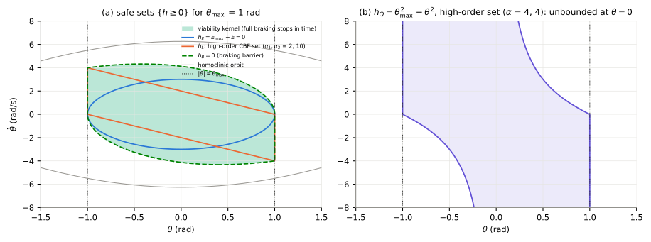
The requirement: keep the swing below an amplitude, \(|\theta| \le \theta_{\max} = 1\) rad. A barrier function \(h\) turns it into a set: the safe set is \(\{x : h(x) \ge 0\}\) [17], [18]. Four barriers express the requirement (or a stronger one) differently:
- Energy, \(h_E = E_{\max} - E\) with \(E_{\max} = -\tfrac{g}{l}\cos\theta_{\max}\): the region inside the unpowered pendulum’s swing of amplitude \(\theta_{\max}\). The input appears directly in its rate, \(\dot h_E = -\dot\theta\,u\) (“relative degree one”).
- Angle, quadratic, \(h_Q = \theta_{\max}^2 - \theta^2\): its rate \(-2\theta\dot\theta\) does not contain \(u\), so a high-order barrier is needed [19]: the condition is imposed on \(\psi_1 = \dot h + \alpha_1 h\), whose rate does contain \(u\).
- Angle, linear, \(h_L = \theta_{\max} \mp \theta\), one per side, each with its high-order barrier (\(\alpha_1 = 2\), \(\alpha_2 = 10\)).
- Braking, \(h_B\): built from the motion full braking produces. Under \(u = -u_{\max}\) the quantity \(E_u = \tfrac12\dot\theta^2 - \tfrac{g}{l}\cos\theta + u_{\max}\theta\) is constant, so \(h_B \ge 0\) exactly when full braking stops the swing before \(\theta_{\max}\) (and its mirror image for the other direction). Full braking always satisfies its condition.
The condition and the safety filter
The condition is \(\dot h(x, u) \ge -\alpha\,h(x)\): the barrier may decrease, but never faster than in proportion to its own value, so it can approach zero and never cross it (\(h(t) \ge h(0)\,e^{-\alpha t}\)). On the pendulum each condition is affine in the one input, \(a(x)\,u \ge b(x)\).
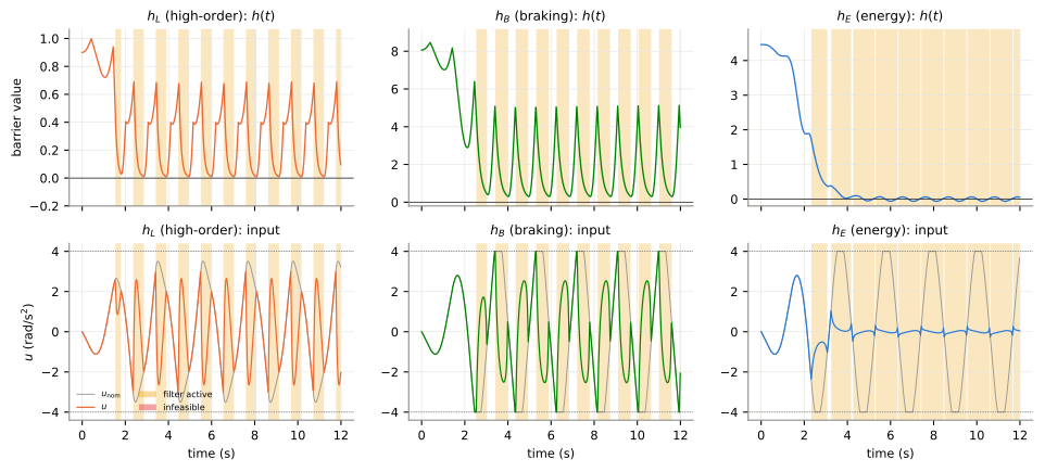
The filter takes the nominal input (the energy pumping) and changes it as little as possible: \[ \min_u\ (u - u_{\text{nom}})^2 \quad \text{subject to} \quad a_i(x)\,u \ge b_i(x)\ \text{for every barrier}, \quad |u| \le u_{\max}. \] With one input the allowed inputs form an interval, and the answer is \(u_{\text{nom}}\) clipped to it. If the interval is empty, the filter is infeasible. It runs every 10 ms on the sampled state. From \((0.1, 0)\) for 12 s:
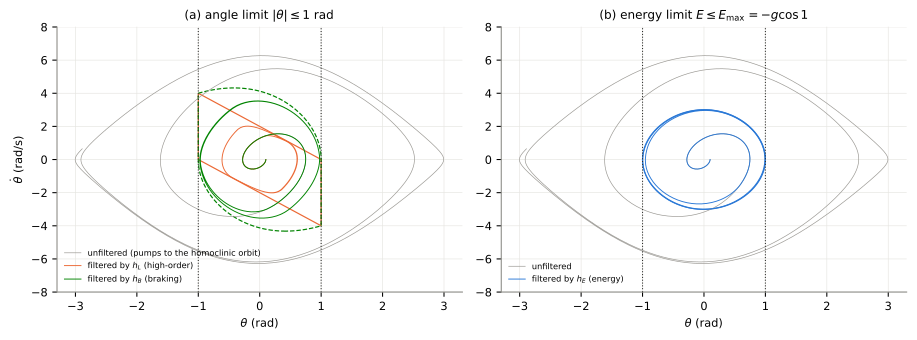
- unfiltered, the pumping reaches the homoclinic orbit and the swing goes over the top;
- filtered by \(h_L\), the swing is held to 0.61 rad: with these \(\alpha\)’s the condition is conservative and stops the pumping well short of the limit;
- filtered by \(h_B\), the swing reaches 0.975 rad, braking hard at each end;
- filtered by \(h_E\), the energy settles at \(E_{\max}\) and the swing at 0.998 rad. Its smallest \(h_E\) is \(-0.066\): the continuous-time condition, applied every 10 ms, lets the sampled system overshoot slightly. That is why the project states its barriers in discrete time, \(h(x_{k+1}) - h(x_k) \ge -\gamma\,h(x_k)\) [20].
No step of these runs was infeasible.
Input limits and feasibility
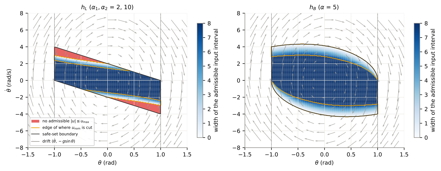
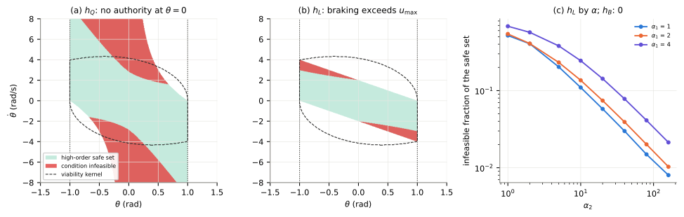
The filter assumes that an admissible input meeting the condition exists. With \(|u| \le u_{\max}\) it may not: there can be “safe” states from which every admissible input leads out. The viability kernel is the largest set from which staying safe is possible; a barrier whose safe set reaches outside it promises what no input can deliver.
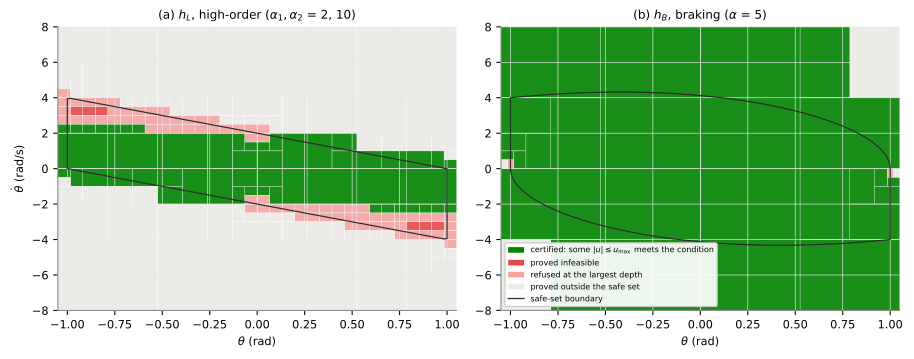
- \(h_Q\) is degenerate. Its gradient vanishes at \(\theta = 0\), so the input’s coefficient vanishes there too, and fast states at the bottom have no admissible input: 8.9 of the safe set’s 23.7 (rad·rad/s) are infeasible. A barrier’s gradient must not vanish where the condition is needed.
- \(h_L\) asks for more braking than the motor has at the corners of its set: a state near one limit moving fast toward it is “safe” by the condition, but cannot be stopped in time. 1.09 of its 8.0 is infeasible. Tuning \(\alpha_1, \alpha_2\) shrinks this (to 0.010 at \(\alpha_2 = 160\)) but never to zero, because gravity at the limit (\(g\sin 1 = 8.25\)) exceeds \(u_{\max} = 4\).
- \(h_B\) is feasible everywhere in its set, by construction: its safe set is the viability kernel (up to the time step), and full braking is always admissible. Building a barrier from the motion of a fixed backup input is the backup-controller construction [21].
The lesson: choose the safe set so that the condition stays feasible under the input limits; the most reliable way is to build it from a motion a fixed admissible input produces, or from a quantity the unpowered system conserves.
Verifying a barrier over sets
The filter checks the condition at the current state only. A certificate proves, over a whole set, that at every state some admissible input meets it. The script does this with the certifier’s own enclosures and branch and prune over the box \([-1.05, 1.05] \times [-8, 8]\). Each piece of the box ends up in one of four classes:
- outside: some barrier is proved negative on all of it, so there is nothing to show;
- certified: an admissible input is proved to meet the condition at every state of the piece’s part of the safe set (for \(h_B\), full braking on one side of \(\dot\theta = 0\) makes that side’s condition hold identically, and the other side’s is proved by its enclosure);
- proved infeasible: the piece lies in the safe set and no admissible input can meet the condition anywhere in it;
- otherwise it is split, and at depth 10 refused.
For \(h_L\): certified 7.6, refused 2.4 and proved infeasible 0.20 (rad·rad/s), the refused and infeasible pieces along the infeasible corners and the set’s edge. For \(h_B\): certified 31.4 and refused 0.03, two tiny pieces at the corners \((\pm 1, 0)\) where the condition is tight.
Two caveats. The condition verified here is the continuous-time one; the discrete-time form is checked the same way with the step map in place of the derivative. And a certificate needs a model: the residual \(\mathcal W\) enters as a disturbance, and what is then certified is input-to-state safety [22], the invariance of a safe set enlarged by the residual’s effect.
Energy shaping with a barrier on top
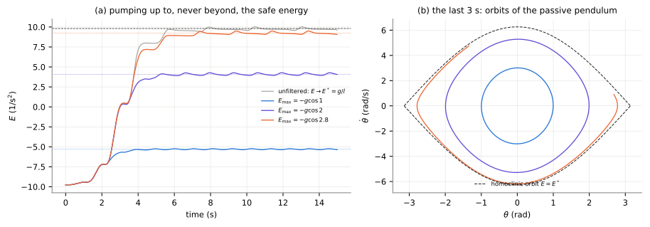
With \(h_E\), the filter turns “pump up to the homoclinic orbit” into “pump up to \(E_{\max}\), never beyond”. For amplitudes of 1, 2 and 2.8 rad the energy settles within 0.26 of \(E_{\max}\). Every safe set \(\{E \le E_{\max}\}\) with \(E_{\max} < E^*\) is bounded by a swing of the unpowered pendulum, so it is invariant with \(u = 0\), and the condition is feasible everywhere in it, whatever \(u_{\max}\) is. As \(E_{\max} \to E^*\) the boundary approaches the homoclinic orbit; beyond \(E^*\) the set contains rotations over the top, and an energy barrier can no longer limit the angle. This is the dissipativity view: a storage function whose sublevel sets the uncontrolled system keeps is a barrier for free. See Background: dissipation certificates.
On the lift: the landing’s barriers. The landing (the block carried up over the step corner and set down on the step) is checked as barrier conditions in two phases.
- The controlled phase: feasibility along the path. While the disk can still push, a disk force within its limits must exist, at every pose along the landing, that keeps every barrier \(h_i \ge 0\) with \(\dot h_i \ge -\alpha(h_i)\). This is the pendulum’s feasibility question, with the disk’s force limits in place of \(|u| \le u_{\max}\); the quasi-static condition “a balancing force exists” is its special case at zero speed. Each \(h\) and \(\alpha\) comes from a physical limit or a measurement, not a tuned value. The hard barriers are:
- the block’s spin rate stays bounded;
- the disk’s penetration into the block stays within its measured band;
- the block stays on the step;
- the disk stays away from the block’s corners: the distance of the disk’s contact point from the ends of the face, minus a margin derived from the measured placement and tracking errors. details: issue #73
- The dynamic phase: an energy barrier. From the first pose where no admissible force exists, the barrier is on a storage function, \(h = E_{\text{rest}} - V(x)\): the block’s energy above its landed rest, at touch-down, must be no larger than the level from which it is certified to come to rest on the step. This is the pendulum’s \(h_E\): a level of a storage function that the dissipative, unpowered motion keeps.
A simple screen of this second kind already runs on executed landings: it rejects a landing whose peak kinetic energy exceeds \(m g(\varepsilon_{\text{pen}} + \varepsilon_{\text{on}})\), a small energy budget: what the block would gain falling through the contact recognizer’s tolerance band (its penetration limit plus its contact tolerance, 6 mm here). On 1,473 recorded landing states it rejected all 19 unsafe landings and no other, where barriers evaluated on the planned motion did not separate them. details: issue #63
The distinction of this section carries over: a safety filter in the controller is an online mechanism whose guarantees are only as good as the condition’s feasibility; a barrier certificate is a proof over sets on the model, carried to the simulator through \(\mathcal W\) like every other certificate here. Safety filters in general are surveyed in [23]; a barrier filter with a learned residual in its derivative, the barrier counterpart of \(\mathcal W\), is [24].
11. The division of labour
| Job | Tool | Kind of statement |
|---|---|---|
| enclose every state’s motion in a piece | zonotope propagation of the rigid reduced model | proof, given \(\mathcal W\) |
| exclude mode switches | mode conditions over sets, branch and prune | proof |
| chain pieces | exit set inside the next entry set | proof |
| bound the model–simulator gap | one-step residuals along simulator rollouts | 95/95 statistics |
| validate the combination | held-out simulator rollouts | counts, with confidence bounds |
| screen candidates fast | batched simulator rollouts | estimate, no certificate |
The statistics go to the smallest, most reusable place, the simulator’s one-step residual, and everything else is proved. Simulator rollouts remain the right tool for a fast screen, not for certificates.
Further reading
- Zonotopes and their reduction: Girard [4]; set arithmetic in JAX with immrax [2]; affine arithmetic [3].
- Tubes around orbits and their composition: maneuver regulation [5], transverse coordinates [6], [7], sequential composition of funnels [8].
- The swing-up law: Åström and Furuta [1].
- Statistics: Wilks’ tolerance limits [13]; the scenario approach [10].
- Control barrier functions: Ames et al. [18], high-order barriers [19], backup sets [21], discrete time [20], safety filters [23].
- Related ways to bridge a model and a simulator: simulation-gap functions [14], reachset conformance [15], smoothing-error tubes for contact [25].
On this site: Background: zonotope propagation, Background: certified funnels and composition, Background: control barrier functions, Certified funnels.