Climbing a Hill You Cannot See

Gradient estimation for wind turbine control, and five things nobody has settled

Aykut C. Satici

Robot Control Lab · Systems Engineering · UT Dallas

Two regimes, one optimization problem
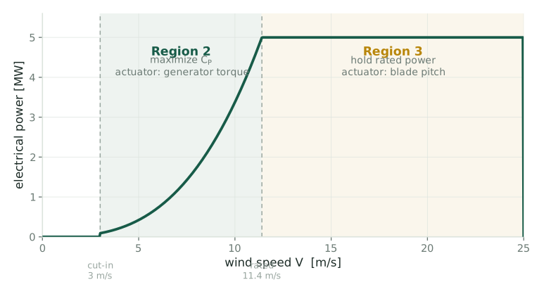
Power curve of a 5 MW turbine. Between cut-in at 3 m/s and rated at 11.4 m/s, power rises as the cube of wind speed; above rated it is held flat at 5 MW.

Region 3: above rated

There is more wind than the machine can use. Throw the excess away and hold rated power. A setpoint, an error signal and a PI controller.

Region 2: below rated

Take everything the wind offers. There is no setpoint, only an efficiency to maximize. This is the only regime containing an extremum to seek.

The hill
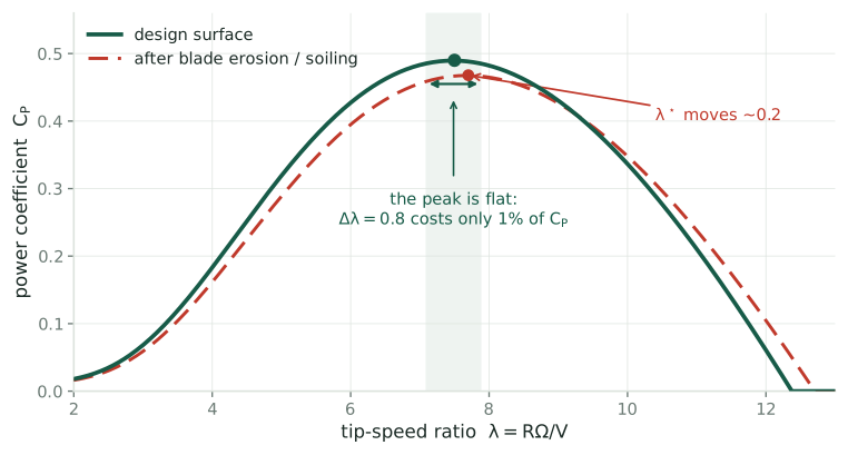
Power coefficient versus tip-speed ratio. A single smooth peak of 0.49 at lambda 7.5, steep on the left and gentle on the right. A dashed red curve shows the same rotor after erosion: peak lower and shifted right by 0.2.

The rotor’s efficiency depends on one number, the tip-speed ratio \(\lambda = R\Omega/V\), which is blade tip speed divided by wind speed. Hold \(\lambda\) at \(\lambda^\star\) and you capture the most power available.

You cannot measure either axis
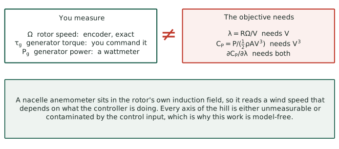
Left box: measurable signals are rotor speed, generator torque and generator power. Right box: the objective needs lambda and C_P, both of which require the wind speed. They are not equal.

Both coordinates of the hill are written in terms of \(V\), the wind speed actually reaching the rotor, which is exactly what a turbine cannot measure.

Sitting on a hill you cannot see

How the controller finds the peak without measuring where it is.

The \(k\Omega^2\) law

The generator is commanded to resist the rotor with a torque quadratic in speed,

\[\tau_{\text{gen}} = k\,\Omega^2 .\]

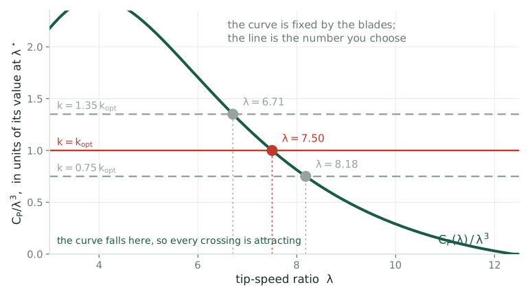
Balance it against the aerodynamic torque \(T_{\text{aero}} = \tfrac12\rho\pi R^3V^2\,C_Q(\lambda)\), with \(C_Q = C_P/\lambda\), and the equilibrium condition is

\[\boxed{\ \frac{C_P(\lambda)}{\lambda^3} \;=\; \frac{2k}{\rho\pi R^5}\ }\]

The wind speed cancels. Try \(\tau_{\text{gen}} = k\Omega^n\) and you get \(C_Q(\lambda)/\lambda^{n} \propto V^{\,n-2}\). Only \(n = 2\) removes \(V\), so it is the unique exponent for which the equilibrium tip-speed ratio does not depend on the wind.

There is no rotor speed to regulate to
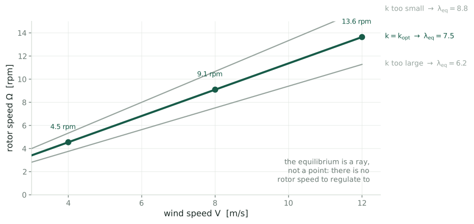
Rotor speed versus wind speed. Three straight lines through the origin, one per torque gain. The middle line is the optimal one; points on it at 4, 8 and 12 m/s show three different rotor speeds.

The equilibrium of the rotor equation is a ray, not a point. Every wind speed gets its own \(\Omega\); all of them share the same \(\lambda\). The controller never rejects the wind. It makes the desired behaviour an attracting manifold and lets the wind slide the machine along it.

So the problem reduces to one number

What we have

A single scalar knob \(k\), and a monotone map from \(k\) to the tip-speed ratio the machine settles at.

What we want

The \(k\) that lands us on the peak. The factory value is wrong at commissioning and gets worse as the blades age.

Find the maximum of a function you cannot evaluate, by turning a knob and watching a noisy meter. That is extremum seeking control, and it is what the last decade of work at UTD has been about.

Extremum seeking

Estimate a derivative you cannot measure by wiggling the input.

The loop

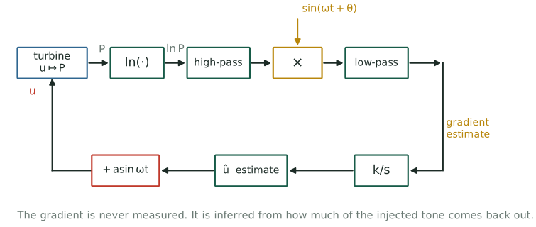
Block diagram: the control parameter enters the turbine, power comes out, is passed through a logarithm, high-pass filtered, multiplied by a phase-shifted copy of the dither, low-pass filtered, and integrated back onto the parameter.

Add a slow sinusoid \(a\sin\omega t\) to the knob. If the output wiggles in phase, you are on the uphill side; out of phase, the downhill side. Multiply and average, and what survives is proportional to the slope.

The one identity that made it practical

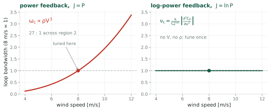
Power is proportional to the cube of the wind speed, so the gradient of power is too, and the wind varies by 3:1 across Region 2. A loop tuned at 8 m/s is 27 times too slow at 4 m/s and 27 times too aggressive at 12 m/s.

Rotea’s 2017 observation is one line. Since \(\ln P = \ln(\tfrac12\rho A) + 3\ln V + \ln C_P(u)\), and the wind term does not depend on \(u\):

\[\frac{\partial \ln P}{\partial u} \;=\; \frac{1}{C_P}\frac{\partial C_P}{\partial u}\]

Feed the algorithm \(\ln P\) instead of \(P\) and the loop bandwidth becomes \(\nu_c = (\kappa/C_P^{\max})\,|\partial^2 C_P/\partial u^2|\), free of both the wind speed and the air density. Tune it once; it works everywhere.

What the logarithm fixes

Two panels. Left, power feedback: loop bandwidth rises as the cube of wind speed, spanning 27 to 1. Right, log-power feedback: a flat line.

It holds up in high-fidelity simulation
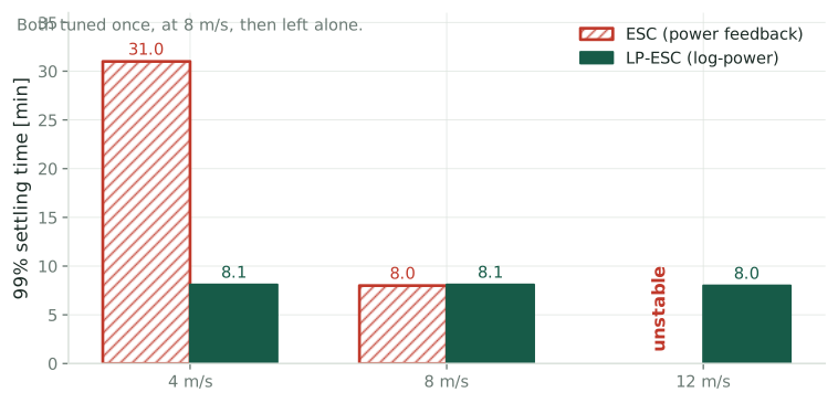
Bar chart of settling time at 4, 8 and 12 m/s under shear and 10 percent turbulence. Plain ESC takes 31 minutes at 4 m/s, 8 minutes at 8 m/s, and is unstable at 12. Log-power ESC takes about 8 minutes at all three.

Ciri, Leonardi & Rotea 2019

Large-eddy simulation of the full flow around an NREL 5 MW rotor, with shear and 10% turbulence. No analytic gradient anywhere.

The result

Log-power holds 8 minutes across a 3:1 wind range. Plain ESC is four times slower at the bottom and goes unstable at the top.

Making it fast: LP-PIESC
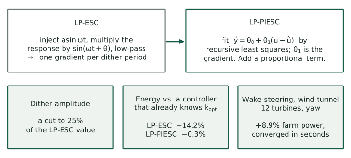
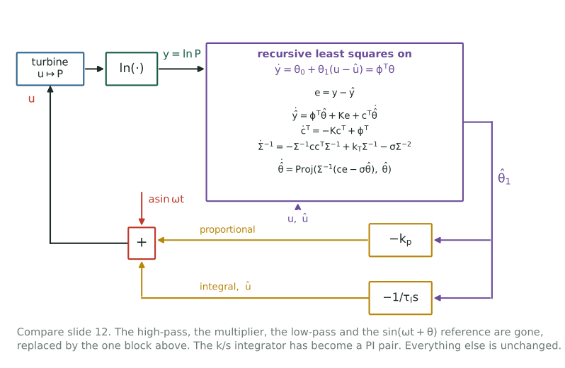
Comparison: LP-ESC demodulates a dither; LP-PIESC fits a two-parameter model by recursive least squares. Three result cards: smaller dither, energy loss cut from 14.2 to 0.3 per cent, and 8.9 per cent farm power gain in a wind tunnel.

Replace demodulation with recursive least squares on \(\dot y = \theta_0 + \theta_1(u-\hat u)\) and add a proportional term. The gradient \(\theta_1\) now comes with a covariance matrix \(\Sigma\) that the algorithm already propagates, and that none of these papers reports.

Where things stand

Solved

Consistency across wind speed. The logarithm removes the \(V^3\) dependence exactly, in theory, in LES, and in the tunnel.

Solved

Speed. LP-PIESC converges fast enough that the search costs 0.3% of energy rather than 14%.

Not solved

Everything to do with noise. “The enemy is process noise”, and none of these papers reports a variance.

Extremum seeking works well when the process noise is negligible. Otherwise you must average, and averaging costs convergence time. That trade-off has not been quantified for this problem.

Five things nobody has settled

Each one is a well-posed question with an answer somebody could get.

Q1 · What is the estimator estimating?

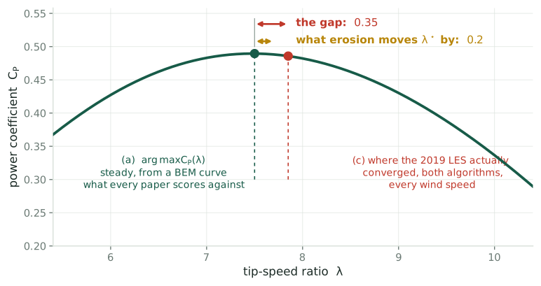
The C_P curve near its peak. A green marker at lambda 7.5 labelled the steady BEM optimum; a red marker at 7.85 where the 2019 LES actually converged. The 0.35 gap between them is drawn against the 0.2 shift that blade erosion produces.

In the 2019 LES, both algorithms converge to \(\bar\lambda \approx 7.85\) against a design value of \(7.5\), at every wind speed, in every condition. The paper calls this “close to the ideal optimum” and moves on.

Q1 · Why it is a variance problem

Time series over ten minutes. The wind contribution to log power swings with standard deviation 0.30 nepers; the turbine's response to the probe is a small clean sinusoid of amplitude 0.02.

\(3\ln V\) is independent of the knob, so it vanishes from the gradient exactly. It does not vanish from any finite-time estimate of that gradient, and it is fifteen times larger than the signal.

Q1 · The trade that was never computed

Log-log plot of mean-square error against dither amplitude. Bias squared rises as the fourth power; variance falls as the inverse square; the sum has a clear minimum. Vertical lines mark the amplitudes chosen in the two published papers.

A central difference estimates \(J'(q) + \tfrac{a^2}{6}J'''(q)\), so its zero sits off the true optimum by \(-\tfrac{a^2}{6}\,J'''/J''\). Bigger dither, less noise, more bias. There is an optimal \(a\), and both published values were chosen by trial and error.

Q2 · What sets the stability limit?

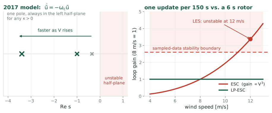
Left: the 2017 model has a single pole on the negative real axis that just moves further left as wind speed rises, so it can never go unstable. Right: loop gain versus wind speed crossing a sampled-data stability boundary, with the LES instability at 12 m/s marked.

The 2017 model is first order: \(\dot{\tilde u} = -\omega_c\tilde u\). It cannot go unstable for any positive gain. The LES did, twice: in uniform flow and in turbulence.

Q3 · Does the turbine need to probe at all?

The rotor equation is \(I\dot\Omega = T_{\text{aero}} - \tau_{\text{gen}}\). Every term on the right is known: \(\tau_{\text{gen}}\) is commanded, \(\Omega\) is measured, and \(I\) is a design constant. So

\[T_{\text{aero}}(t) \;=\; I\dot\Omega(t) + \tau_{\text{gen}}(t)\]

is exactly reconstructible without any anemometer. And turbulence already swings \(\lambda\) between 6 and 8.5 all day long, for free.

The dither exists because the excitation is unknown, not because excitation is lacking. So: are \(V(t)\) and the curve \(C_Q(\cdot)\) jointly identifiable from the record of \((\Omega,\,T_{\text{aero}})\) alone?

Q3 · Exactly one blind direction

Left: two different C_P curves, one a rescaled copy of the other. Right: both produce an identical aerodynamic torque record, so the data cannot distinguish them.

Substituting \(\tilde V = cV\) into \(T_{\text{aero}} = \tfrac12\rho\pi R^3V^2C_Q(R\Omega/V)\):

\[\tilde C_Q(x) = \frac{C_Q(cx)}{c^2} \quad\Longrightarrow\quad \tilde C_P(x) = \frac{C_P(cx)}{c^3} \quad\Longrightarrow\quad \tilde\lambda^\star = \frac{\lambda^\star}{c}\]

There is one unidentifiable direction, an overall scaling of the wind, and it maps straight onto a scaling of \(\lambda^\star\). Everything else about the curve is determined. Air density errors, by contrast, scale \(C_P\) uniformly and do not move the peak.

Q4 · What the curvature is doing

Look again at the 2017 result:

\[\nu_c \;=\; \frac{\kappa}{C_P^{\max}}\left|\frac{\partial^2 C_P}{\partial u^2}(u_o)\right|\]

Choosing the gain \(\kappa\) to hit a target settling time requires the curvature at the peak, currently taken from a design curve that the LES says is wrong by 10% in \(C_P\). The gain calibration is not self-consistent, and “it takes too long to tune” is partly a symptom of that.

The curvature also sets the terminal scatter, \(\sigma_\lambda \approx \sigma_{\hat g}/|H|\), and the energy lost to mistuning is quadratic in \(\sigma_\lambda\). The same number sets the gain, the achievable accuracy and the cost of missing.

Q4 · Two routes to the same covariance
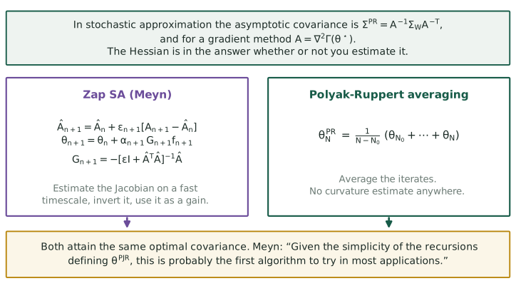
Top: the asymptotic covariance in stochastic approximation is A-inverse Sigma A-inverse-transpose, and A is the Hessian. Below, two boxes: Zap stochastic approximation estimates the Jacobian and inverts it; Polyak-Ruppert averaging simply averages the iterates. Both reach the same optimal covariance.

Meyn does not estimate the Hessian in the ESC papers. It appears in the analysis, as the matrix \(A = \nabla^2\Gamma(\theta^\star)\) governing the asymptotic covariance. Where he does estimate it, in Zap SA, it is a two-timescale recursive Jacobian estimate used as a matrix gain: stochastic Newton-Raphson.

Q5 · How good could any algorithm be?
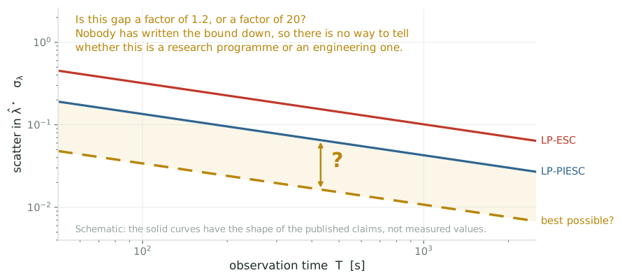
Log-log schematic of terminal scatter against observation time. Two solid curves for the published algorithms and a dashed gold curve far below them labelled best possible, with the gap between them marked by a question.

Given a turbulence spectrum, an observation time and a fatigue budget, how well can anyone locate \(\lambda^\star\)? Nobody has written the bound down.

Why turbulence is not ordinary noise

In classical stochastic approximation

Noise is pure nuisance. It corrupts the measurement and you average it away.

Here

Turbulence is simultaneously the noise and the excitation. It is what corrupts the gradient estimate and what sweeps the rotor across the curve for free.

That duality is what the stochastic-approximation literature does not cover, and it is what makes Q3, estimating the curve without probing it, plausible.

The experiment I would run first

Take the existing simulation setup. Run it at two or three dither amplitudes, with several independent, non-repeating turbulence seeds. Look at where the torque gain lands.

If the offset scales as \(a^2\)

It is estimator bias. The algorithm is systematically missing the peak, and the fix is a known one.

If it is flat in \(a\)

The turbulent optimum has moved, and the published results have been scored against a reference that is off.

Either way the seed spread yields \(\sigma(\hat g)\) and \(\sigma_\lambda\), which none of these papers reports. Two outcomes, both publishable, a few days of compute.

Climbing a hill you cannot see

The algorithms work. What is missing is the statistics of the quantity they compute.

What exists

A model-free loop, consistent across wind speed and fast enough to deploy, with results from large-eddy simulation, a wind tunnel and a field test.

What does not

A definition of the estimand, a variance for it, an account of the stability limit, a performance bound, and an answer on whether the dither is needed.

Rotea, IFAC 2017 · Ciri, Leonardi & Rotea, Wind Energy 2019 · Kumar & Rotea, Energies 2022 · Rotea et al., TORQUE 2024 · Lauand & Meyn, IEEE CSM 2023

Prepared for a collaboration with M. A. Rotea, UTD Wind Energy Center.