Gradient Noise in Extremum Seeking for Wind Turbines

How turbulence sets the power that LP-ESC and LP-PIESC lose, and the tuning that loses least

Aykut C. Satici

Robot Control Lab · Systems Engineering · UT Dallas

The result in brief

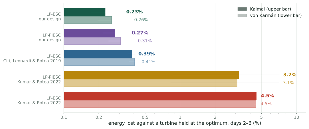
41% less energy lost than the best published design, LP-ESC of Ciri, Leonardi & Rotea 2019 (same one-day tracking time): 0.385% → 0.227%, about 27 MWh per turbine-year at 8 m/s

14× less than the LP-PIESC of Kumar & Rotea 2022: 3.19% → 0.227%, about 500 MWh per turbine-year

20× less than the LP-ESC tuning of Kumar & Rotea 2022: 4.51% → 0.227%, about 730 MWh per turbine-year

Six-day simulations of the nonlinear NREL 5 MW turbine at 8 m/s, turbulence intensity 0.10, four wind records per spectrum; every controller runs in the same wind as a turbine held at the optimum. Bars: mean over records, lines: range. Solid: Kaimal; light: von Kármán.

The headline. Designed from the turbulence spectrum, an ordinary demodulation loop loses 0.23 percent of the energy. The best published design loses 0.39; the two 2022 tunings lose 3 to 4.5 percent. The rest of the talk is where these numbers come from, and why the prediction and the simulation agree.

One gain, unknown and drifting

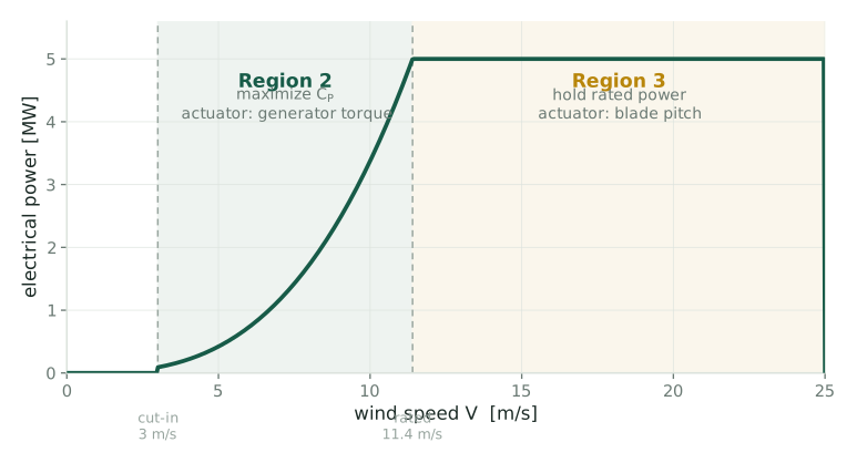
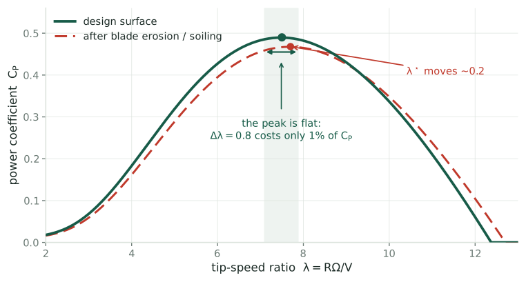
Below rated wind speed the turbine should run at the tip-speed ratio \(\lambda = R\Omega/V\) that maximizes the power coefficient \(C_P(\lambda)\). The standard controller sets the generator torque to \(u\,\Omega^2\); the gain \(u\) alone fixes where the rotor settles, at every wind speed (Unit 1).

The best gain \(u^\star\) depends on the blades, which erode, ice and foul. It must be found online, and found again when it moves.

At a fixed tip-speed ratio, both torques scale as V squared, so the wind cancels and the gain alone sets lambda. The optimum is one number, but it drifts with the blades.

Extremum seeking finds it, by two routes

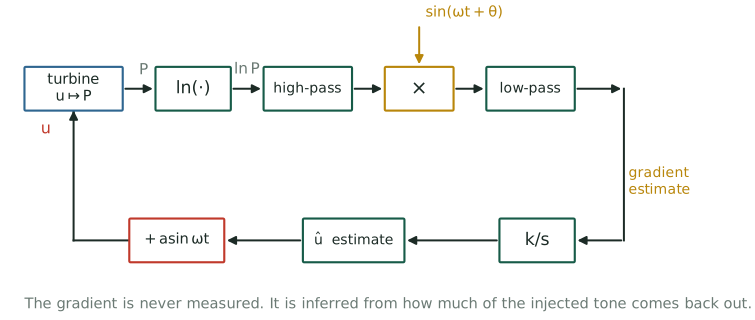
1. Dither: add \(a\sin\omega t\) to the gain, period \(T = 2\pi/\omega\).
2. Estimate: read from log-power \(y = \ln P\) how power changes with the gain.
3. Step: move the gain uphill, once per period (step size \(\kappa\)) or continuously.

LP-ESC: demodulation Correlate \(y\) with the dither over each period: the in-phase channel \(\hat g\) [Rotea 2017; Ciri, Leonardi & Rotea 2019].

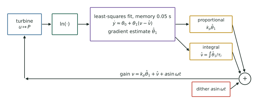
LP-PIESC: least squares Fit \(\dot y \approx \theta_0 + \theta_1(\nu - \hat\nu)\) by recursive least squares; proportional-integral update [Kumar & Rotea 2022].

Both are log-power schemes: the log removes the mean wind speed from the loop gain. They differ in how they turn the response into a gradient.

LP-PIESC: a least-squares fit in place of the correlation

Published tuning [Kumar & Rotea 2022]: \(T = 314\) s, \(a = 0.082\,\nu^\star\), estimator memory \(1/k_T = 0.05\) s, ridge \(q = 10^{-6}\), \(k_p = 5\times10^{-6}\) s, \(\tau_I = 2.8\); normalized gain \(\nu = 0.061\,u/u^\star\). Reported to reach the optimum almost at once, with a quarter of the classical dither.

Keep in mind two numbers: a memory of a twentieth of a second, and a period of five minutes. Their ratio is what decides what this estimator reads.

Turbulence makes the gain scatter

Scatter \(\sigma(\tilde u)\): the standard deviation of the gain error \(\tilde u = u - u^\star\) once the loop has settled, a spread over time quoted as a fraction of \(u^\star\). It concerns the center of the dither only; the dither’s own cost is counted separately. Every excursion costs power: the loss is \(\tfrac12|J''|\,\sigma(\tilde u)^2\) plus the dither’s cost.

Left: the 2022 LP-PIESC in four wind records over six days, started at the optimum. It random-walks. Right: our design, same winds. The scatter is the size of this motion.

What this work answers

Given the wind’s spectral density and the tuning of each controller:

1. How noisy is one gradient estimate at the optimum, and what does LP-PIESC’s estimate measure?
2. How large is the scatter of the gain in steady state?
3. How much power is lost, and which tuning loses least for a required tracking time?
4. How do the two routes compare, and do the predictions survive simulation, including the published runs?

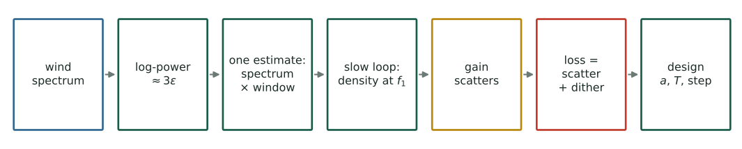
The answer in one line. At the optimum the wind enters log-power as \(3\varepsilon\), so each estimate is the wind seen through a known window; a slow loop sees only the wind’s density at the dither frequency; the scatter, the loss and the best tuning then follow in closed form from three numbers: that density, the curvature of \(C_P\) at its peak, and the rotor time constant.

Everything that follows is this one sentence, unpacked and checked.

The argument in one line

The wind \(\Phi(f_1)\): the turbulence density at the dither frequency \(f_1 = 1/T\) (IEC Kaimal or von Kármán).

The rotor \(\tau_r = 6.88\) s: the time constant with which the rotor follows the gain (at 8 m/s).

The power curve \(\chi = 6.3\): how sharply \(C_P\) peaks; \(|J''(u^\star)|\,u^{\star2} = \chi/9 = 0.70\).

Five links, each checked in simulation. Then the design, and the evidence on energy.

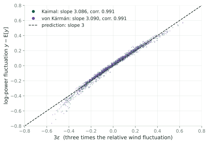
Link 1: at the optimum, the wind enters log-power as \(3\varepsilon\)

With \(V = \bar V(1 + \varepsilon)\), power is \(\propto V^3 C_P(\lambda)\), so \[y = \ln P = \text{const} + 3\ln(1+\varepsilon) + \ln C_P(\lambda).\]

At \(u^\star\) the power curve is flat: \(C_P'(\lambda^\star) = 0\), so the wind’s effect through \(\lambda\) drops out at first order, and \[y - \mathbb{E}[y] = 3\,\varepsilon + O(\sigma_\varepsilon^2).\]

Simulation: slope 3.086 (Kaimal), 3.090 (von Kármán); correlation 0.991.

A gust changes power only through the cube of the wind speed, because at the peak the power curve is flat. That single term makes everything else linear.

Link 2: one estimate sees the spectrum through a window

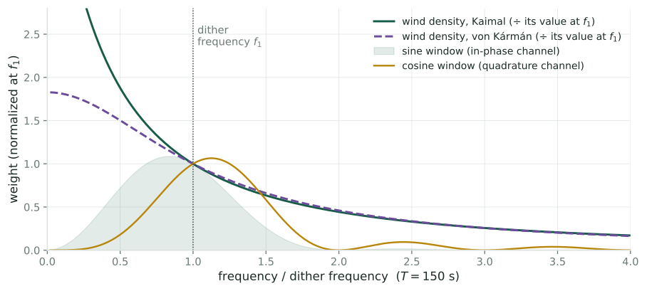
The demodulated estimate correlates \(y\) with \(\sin\omega t\), so its noise is \(6Z_n/(aT)\) with \(Z_n = \int_0^T \varepsilon(nT+t)\sin\omega t\,dt\), and \[\operatorname{Var}(Z) = \int \Phi(f)\,|\hat w(f)|^2\,df .\]

Both windows pass \(f_1\) equally; the sine window leans to low frequencies, where the wind has its energy, so the quadrature (cosine) channel is the quieter one per estimate (Units 12–14).

A linear filter of a stationary wind: its variance is the spectrum integrated against the filter’s squared gain.

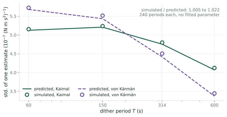
Checked over a tenfold range of dither periods

Predicted and simulated standard deviation of one estimate agree within 0.5 – 2.2 % for \(T\) from 60 to 600 s under both spectra, with no fitted parameter; the small excess is the size and sign of the terms the prediction leaves out.

240 periods per point; sampling uncertainty about 4.6 percent per point.

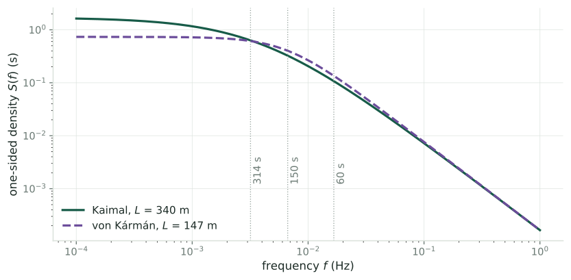
The two IEC turbulence spectra

• Same flat level \(4\sigma_\varepsilon^2 L/\bar V\), so \(L\) is the integral length scale: 340 m (Kaimal), 147 m (von Kármán) at the 90 m hub.
• Both fall as \(f^{-5/3}\); they differ mainly near their corners.
• At the published period (314 s) the densities agree within 3 %; at 60, 150, 600 s their ratio is 0.79, 0.81, 1.35.
• Effect on the predicted scatter: at most 11 % over 60–314 s. No conclusion changes.

Everything is worked out twice, on equal footing. The spectrum enters only through its value at the dither frequency.

Link 3: the published LP-PIESC reads the quadrature channel

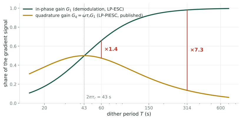
Over a 0.05 s memory the regressor is frozen, so the ridge fit returns the minimum-norm product \[\hat\theta_1 = \frac{d\,\dot y}{1 + d^2 + \gamma},\] whose period average is the cosine (quadrature) coefficient of \(y\). Its signal is \(G_q = \omega\tau_r G_1\): 0.135 against 0.981 for demodulation at 314 s.

Simulation: \(\hat\theta_1\) follows \(d\,\dot y\) with correlation 0.997; in-phase / quadrature 7.24, predicted \(1/(\omega\tau_r) = 7.27\).

The estimator sees the gradient only through the rotor’s lag. A rotor without lag would give it no gradient signal at all.

Link 4: a slow loop sees one frequency

Averaging \(N\) estimates is one estimate over \(N\) periods; its window narrows onto \(f_1\) (Fejér). So the noise a slow loop feels is the long-run variance \[\sigma_\infty^2 = \frac{2\Psi}{a^2T},\qquad \Psi = 9\,\Phi(f_1),\] and the scatter at tracking time \(\tau_c\) is \[\sigma(\tilde u)^2 = \frac{\Psi}{a^2 g^2\,\tau_c\,J''^2},\quad g = G_1 \text{ or } G_q .\]

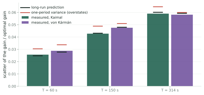
Simulated loops: within 4 % of the long-run prediction; one period’s variance overstates by up to 18 %.

The period cancels from the scatter once you fix the tracking time; the wind enters through its density at one frequency.

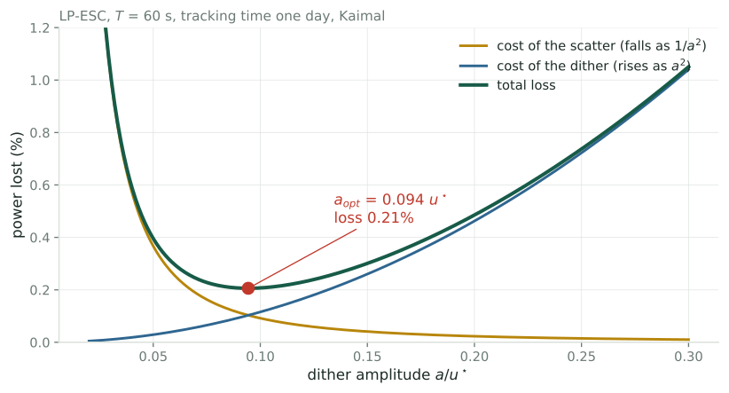
Link 5: loss = scatter + dither; the best amplitude balances them

\[\ell(a) = \underbrace{\frac{\Psi}{2a^2g^2\tau_c|J''|}}_{\text{scatter}} + \underbrace{\tfrac14|J''|G_1a^2}_{\text{dither}}\]

Least when the two are equal: \[a_{opt} = \Big(\frac{2\Psi}{g^2G_1\tau_cJ''^2}\Big)^{1/4},\qquad \ell_{min} = \sqrt{\frac{\Psi G_1}{2\tau_c g^2}}.\]

Then \(\kappa = T/(\tau_c G_1|J''|)\) (LP-ESC) or \(\tau_I = \tau_c\pi a^2G_q|J''|/T\) (LP-PIESC).

A larger dither lets a loop of fixed tracking time take smaller steps and scatter less, but the dither itself costs power. The least loss balances the two.

Choosing the period

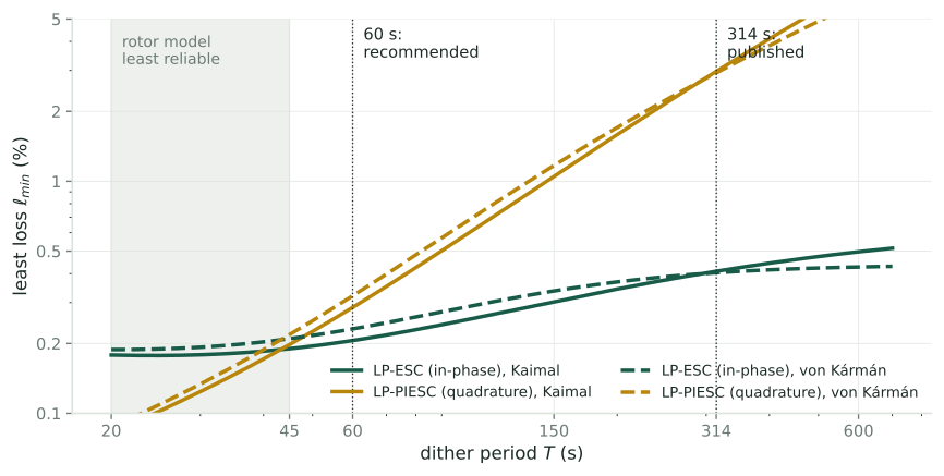
Shorter periods move \(f_1\) up the falling spectrum, so the least loss falls, until the rotor’s lag takes over. Recommendation: \(T = 60\) s (about nine rotor time constants): LP-ESC 0.21 %, LP-PIESC 0.29 % (Kaimal, one day), against 0.41 % and 2.98 % at 314 s. The quadrature penalty \(1/(\omega\tau_r)\) falls from 7.3 to 1.4.

Below about 45 seconds the static power curve and the first-order rotor are least reliable, so we stop at 60.

The published LP-PIESC tracks in 5.1 days

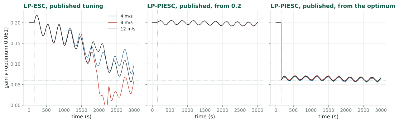
Its integral path is a slow loop on the quadrature channel with loop gain \(7.13\times10^{-4}\) per period: tracking time 5.1 days, stationary scatter 0.33 \(u^\star\), loss 3.9 % (Kaimal). The published fast convergence appears only when the integrator starts at the optimum, which the closed-form optimum makes possible.

LP-ESC with its published tuning converges in about 1000 seconds, as reported. LP-PIESC barely moves from any other start in 3000 seconds.

Energy over six days, every controller in the same wind

controller (\(T\), \(a/u^\star\))	Kaimal, days 2–6	predicted	von Kármán, days 2–6	predicted
LP-ESC, Kumar & Rotea 2022 (314 s, 0.33)	4.51 %		4.48 %
LP-PIESC, Kumar & Rotea 2022 (314 s, 0.082)	3.19 % (0.9–7.1)	3.9 %a	3.09 %
LP-ESC, Ciri, Leonardi & Rotea 2019 (150 s, 0.136)	0.385 %	0.38 %	0.406 %	0.39 %
LP-PIESC, our design (60 s, 0.111)	0.275 %	0.29 %	0.308 %	0.32 %
LP-ESC, our design (60 s, 0.094)	0.227 %	0.21 %	0.258 %	0.23 %

Energy lost against a turbine held at \(u^\star\) in the same wind; mean of four six-day records. ^a stationary prediction for a 5.1-day tracking time, which six days do not reach. Our designs and the 2019 design use a one-day tracking time.

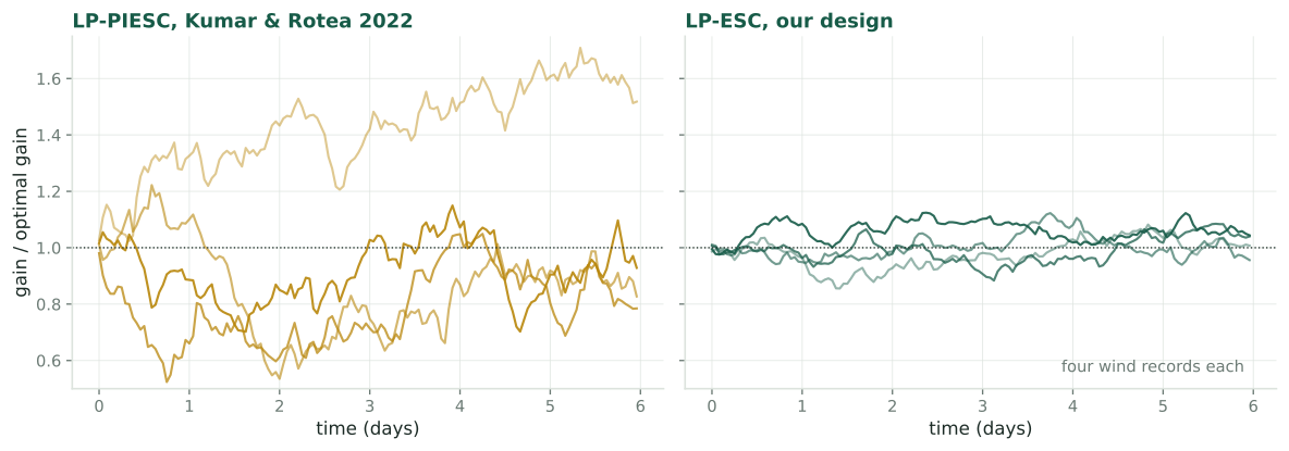
The designs lose what the formulas predict. The 2022 LP-PIESC depends on the wind record (0.9 to 7.1 %); the 2022 LP-ESC loses 1.94 points to its large dither alone.

Every number here is in the claim checker. The prediction for the designs comes from three numbers and was made before the simulation.

After the optimum moves

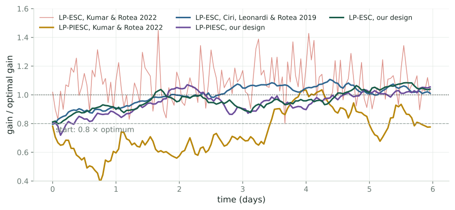
Gain started at 0.8 \(u^\star\). Energy lost on the first day: our LP-ESC 0.67 %, LP-ESC 2019 0.89 %, LP-PIESC 2022 3.2 % (0.6 to 9 % with the wind record), LP-ESC 2022 4.2 %. The 2022 LP-PIESC’s gain wanders instead of converging (0.78–1.45 \(u^\star\) after six days).

One wind record shown. The designs return within about a day, as their tracking time says.

Gains over the published designs

−41 % energy lost vs. the best published design (LP-ESC, Ciri, Leonardi & Rotea 2019, same tracking time): 0.16 points, 27 MWh per turbine-year at 8 m/s. Von Kármán: −36 %.

÷14 vs. LP-PIESC, Kumar & Rotea 2022: 2.97 points, 508 MWh per turbine-year. Our LP-PIESC retuned by the same rules: ÷12.

÷20 vs. LP-ESC, Kumar & Rotea 2022: 4.28 points, 733 MWh per turbine-year, 1.94 points of it the large dither alone.

Remark. Measured in our simulator: NREL 5 MW rotor with a static power curve and a first-order rotor, aerodynamic power, 8 m/s, turbulence intensity 0.10, synthesized turbulence. The published designs were tuned in other simulators; the comparison holds turbine, wind and (for the 2019 design) tracking time fixed, so the design is the only difference. Reference turbine: 1.95 MW mean, 17.1 GWh per year at this wind.

The gain over the best published design comes entirely from the period and the amplitude: shorter period, amplitude set where scatter and dither cost the same.

When is LP-PIESC the right choice?

The gap is a tuning choice The penalty comes from the 0.05 s memory plus fitting \(\dot y\). Fit \(y\) itself over a full period and least squares reads the in-phase channel, with demodulation’s loss. At 60 s the published estimator costs only 20 % more (0.275 vs 0.227 %).

Least squares gives more than an estimate An explicit model, an information matrix that can serve as an error bar, and updates in continuous time: useful for a loop that acts on its own uncertainty.

The quadrature channel’s one merit A slow wind drift within a period reads as gradient in the sine window but cancels in the cosine window. It loses more signal (\(\times\omega\tau_r\)) than it saves in noise.

Speed was the published motivation This work measures steady-state loss of a slow loop and neglects the proportional path. Whether a retuned least-squares loop recovers faster after the optimum moves is open.

For steady-state energy capture, choose demodulation or a full-period least-squares fit. Choose LP-PIESC’s structure where its model, its error bar or a faster transient is needed, and tune it by these rules.

The design procedure

Three numbers

1. \(\tau_r = \dfrac{2I\lambda^{\star2}}{3\rho\pi R^4\bar V C_P^{max}}\) from the rotor data.
2. \(\chi\) from the design power curve: \(|J''(u^\star)| = \chi/(9u^{\star2})\).
3. \(\Psi = 9\,\Phi(1/T)\) from the site’s spectrum (or the IEC model).

One choice: the tracking time \(\tau_c\) (blades change over weeks; recover from start-up within a day: \(\tau_c = 1\) day).

Then

4. \(T \approx 9\,\tau_r\) (60 s here).
5. \(a = a_{opt}\).
6. \(\kappa = T/(\tau_cG_1|J''|)\) or \(\tau_I = \tau_c\pi a^2G_q|J''|/T\).

An error in the curvature changes only the tracking time (\(\tau_c|J''_d/J''|\)); the loop stays unbiased.

Everything needed before any simulation is run.

Limits, and the next step

• Stationary wind, fixed mean speed and turbulence intensity; a day mixes wind states.
• Point spectra of the standard; the rotor averages the wind over its disk (affects content above about 0.06 Hz).
• Static power curve and first-order rotor; induced-flow lag and drivetrain outside the model.
• Aerodynamic, not electrical, power: the term \(I\Omega\dot\Omega\) matters when \(\omega\tau_r\) is not small (0.72 at 60 s).
• LP-PIESC: proportional path and projection neglected.
• The simulations use the same spectra as the analysis: they test the derivation, not the wind models.

Next: test the predictions on measured turbine data and electrical power, and measure recovery speed after the optimum moves, where LP-PIESC was meant to excel.

Summary

1. At the optimum the wind enters log-power as \(3\varepsilon\), so each gradient estimate is the wind seen through a known window.
2. A slow loop sees only the wind’s density at the dither frequency; the scatter is \(\sqrt{\Psi/(a^2g^2\tau_cJ''^2)}\).
3. The published LP-PIESC reads the quadrature channel, \(\omega\tau_r\) of the signal, and tracks in 5.1 days.
4. Loss = scatter + dither; the minimum-loss design follows from three numbers, at \(T \approx 9\tau_r\).
5. Measured over six days: 0.23 % lost, 41 % less than the best published design and 14–20× less than the 2022 tunings.

Technical report and workbook: rotea repository, papers/esc-spectral-noise/.

Backup

B1: The rest point, and why the wind cancels

At a fixed tip-speed ratio \(\lambda = R\Omega/V\), aerodynamic torque \(\tfrac12\rho\pi R^3V^2C_P(\lambda)/\lambda\) and generator torque \(u\Omega^2 = u\lambda^2V^2/R^2\) both scale as \(V^2\). The torque balance is wind-free: \[\frac{C_P(\lambda)}{\lambda^3} = c_u\,u,\qquad c_u = \frac{2}{\rho\pi R^5}.\]

For every gain below \(1.86\,u^\star\) there is exactly one rest point, on the branch through \(\lambda^\star\); it is stable, and near it the rotor is first order with time constant \(\tau_r\) (Units 1–2). Log-power at rest is a wind constant plus \(J(u) = \ln C_P(\lambda_{eq}(u))\), which peaks at \(u^\star = 2.23\times10^6\) N m s² with \(J''(u^\star) = -\chi/(9u^{\star2})\) (Unit 3).

B2: The rotor time constant, and the inertia

\[\tau_r = \frac{2I\lambda^{\star2}}{3\rho\pi R^4\bar V C_P^{max}} = 6.88\ \text{s at } 8\ \text{m/s},\qquad \tau_r\propto 1/\bar V.\]

Inertia from the NREL 5 MW blade and hub data, moving each blade to the shaft by the parallel-axis theorem: \[I_{rotor} = 3\cos^2\beta_p\,(I_b + 2r_hS_b + m_br_h^2) + 115\,926 = 3.88\times10^7\ \text{kg m}^2,\] plus the generator, \(97^2\times534\): \(I = 4.38\times10^7\) kg m². The value \(3.54\times10^7\) used in [Kumar & Rotea 2022] omits the hub-radius offset \(r_h = 1.5\) m.

B3: The rotor seen from the gain

A first-order lag with unit static gain and time constant \(\tau_r\), followed by the slope \(J'\). A dither \(a\sin\omega t\) returns as \[\delta y = J'a\,(G_1\sin\omega t - G_q\cos\omega t),\qquad G_1 = \frac{1}{1+(\omega\tau_r)^2},\quad G_q = \omega\tau_rG_1 .\] At 314 s: \(G_1 = 0.981\), \(G_q = 0.135\); at 60 s: \(G_1 = 0.66\), \(G_q = 0.48\). The two cross at \(T = 2\pi\tau_r = 43\) s, where \(G_q = 1/2\) is largest (Unit 4).

B4: The estimate in calm wind

The demodulated estimate is a Fourier coefficient: \(\hat g_n = B_1/a\), \(\hat g^c_n = A_1/a\) (first sine and cosine coefficients of \(y\) over the period). It ignores the mean and every higher harmonic, but a drift within the period reads as gradient (Unit 5).

Its bias: \(\hat g_n = J'(u_n) + \tfrac{a^2}{8}J'''(u_n) + O(a^4)\). At \(a = 0.136\,u^\star\) the loop settles 0.37 % above \(u^\star\), costing about \(5\times10^{-6}\) of the power, against 0.32 % for the dither itself (Unit 6). The error that matters is random.

B5: The wind as a random process

\(V = \bar V(1+\varepsilon)\), \(\varepsilon\) stationary with autocovariance \(\Gamma(\tau) = \mathbb{E}[\varepsilon(t)\varepsilon(t+\tau)]\), \(|\Gamma| \le \Gamma(0) = \sigma_\varepsilon^2 = \mathrm{TI}^2\), and spectral density \(\Phi(f) = \int\Gamma(\tau)e^{-i2\pi f\tau}d\tau\), one-sided \(S = 2\Phi\), \(\sigma_\varepsilon^2 = \int_0^\infty S\,df\) (Units 7–8). Remainders are ranked by RMS in powers of \(\sigma_\varepsilon\); with sixth moments finite, products of \(k \le 3\) filtered winds are \(O(\sigma_\varepsilon^k)\) (Unit 9).

The tip-speed ratio sees the high-passed wind (corner \(1/(2\pi\tau_r) = 0.023\) Hz); its mean stays at \(\lambda^\star\) to second order (Unit 10). In the Kaimal model 72 % of the variance lies below that corner.

B6: The least-squares estimator, unpacked

The recursion computes, at every instant, the minimizer of an exponentially weighted ridge cost with memory \(1/k_T\) (Unit 15). LP-PIESC’s states combine into \(z = \tilde y + c^\top\hat\theta\) with \(\dot z = -k_fz + \dot y\): it regresses low-pass-filtered \(\dot y\) on the equally filtered regressor, effective ridge \(\gamma = qk_f^2 = 4\times10^{-4}\) (Unit 16).

Memory number \(\mathcal M = \omega^2/(k_T^2\gamma) = 0.0025\): the regressor is frozen over the memory, so the fit is the minimum-norm product, whose period average is the quadrature channel (Unit 17). A fit of \(y\) on \([1, d]\) over a full period returns the in-phase channel.

B7: Correlated noise and the long-run variance

A first-order recursion \(x_{n+1} = \alpha x_n + \kappa v_n\) with correlated noise has variance \[\frac{\kappa^2\sigma_v^2}{1-\alpha^2}\Big[1 + 2\sum_{k\ge1}\alpha^k\rho_k\Big],\] and as the loop slows the bracket tends to \(1 + 2\sum\rho_k\), the long-run variance per sample (Units 20–21). Summed in the frequency domain with Fejér’s kernel, it is \(2\Psi/(a^2T)\), for both channels (Unit 22). For Kaimal at 150 s one period’s variance is 1.29× the long-run value (in-phase) and 0.87× (quadrature).

B8: Short records under-measure the scatter

The sample variance of a record is low by the variance of its own mean: \(\mathbb{E}[s^2] = \sigma^2 - \operatorname{Var}(\bar x)\) (Unit 21). For a two-day record of a loop with a six-hour tracking time (eight tracking times), the sample standard deviation is 0.88 of the true one, a 12 % shortfall. The nonlinear comparison of LP-PIESC against demodulation applies this factor to its predictions.

B9: Away from the optimum

Away from \(u^\star\) the rotor adds a high-passed copy of the wind to log-power with weight \(\eta \approx 2.1\,\tilde u/u^\star\). The noise is multiplied by \(|1 + \eta H(f_1)/3|\); for a loop whose scatter is \(0.1\,u^\star\) it changes by about 2 % (Unit 26). The noise model derived at \(u^\star\) holds over the gains a converged loop visits.

B10: The synthesized wind

A sum of cosines with independent uniform phases, amplitudes \(\sqrt{2S(f_k)/D}\): strictly stationary with the target spectrum on its frequency grid. A ten-hour record sampled at 0.5 s lacks 2.7 % of the variance (mostly above the Nyquist frequency), so its turbulence intensity is 9.86 % (Kaimal); it is Gaussian to within an excess kurtosis of −0.002 (Unit 27). Runs under the two spectra share their random phases.

B11: Where the optimum sits in turbulence

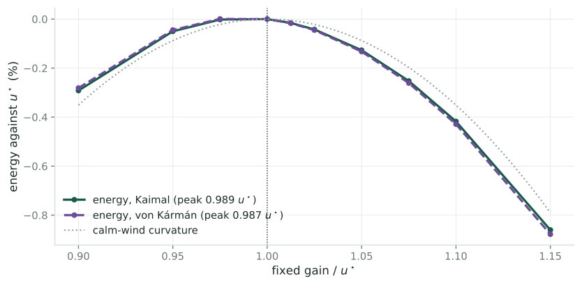
Fixed gains, no dither: the energy peaks at 0.99 \(u^\star\); mean log-power, which the loops climb, at 1.013 \(u^\star\) (1.014 von Kármán). The difference costs about 0.02 % of the energy. The dither alone, centre held at \(u^\star\), costs exactly the calm-wind \(\tfrac14|J''|G_1a^2\): 0.102 % at 60 s and 0.094 \(u^\star\), 0.116 % for the published LP-PIESC dither.

B12: Why the 2022 LP-ESC tuning loses 4.5 %

• Its dither, \(a = 0.33\,u^\star\) at 314 s, costs 1.94 % on its own (measured; the quadratic formula gives 1.88 %).
• Its integrator is fast: it reaches the optimum’s neighbourhood within the first hour, but swings the gain by 0.17 \(u^\star\) root-mean-square, about a mean 10 % above \(u^\star\).
• Together: 4.5 %, steady, independent of the start.

Both it and the 2019 design are LP-ESC; the difference is the tuning.

B13: Simulation setup

turbine	NREL 5 MW rotor, Heier power curve rescaled to \((7.48, 0.4895)\), \(I = 4.38\times10^7\) kg m²
wind	8 m/s, TI 0.10, Kaimal (\(L\) = 340 m) and von Kármán (147 m), synthesized, 0.5 s
integration	adaptive Runge–Kutta (demodulation tests); Euler, 5 ms (LP-PIESC and energy runs)
energy runs	five controllers + reference at \(u^\star\), same wind; 6 days × 4 records × 2 spectra × 2 starts
checks	523 stated numbers recomputed from formulas and stored results by the claim checker

B14: Running example

quantity	value
rotor radius, air density	63 m, 1.225 kg/m³
optimum	\(\lambda^\star = 7.48\), \(C_P^{max} = 0.4895\), \(u^\star = 2.23\times10^6\) N m s² (\(\nu^\star = 0.061\))
curvature	\(\chi = 6.3\), \(|J''(u^\star)|u^{\star2} = 0.70\)
rotor time constant	6.88 s at 8 m/s
dither periods	60 s (recommended), 150 s (2019 design), 314 s (2022 tunings)
tracking time	one day (designs)

References

• [R17] M. A. Rotea, “Logarithmic power feedback for extremum seeking control of wind turbines,” IFAC-PapersOnLine, vol. 50, no. 1, pp. 4504–4509, 2017.
• [CLR19] U. Ciri, S. Leonardi, M. A. Rotea, “Evaluation of log-of-power extremum seeking control for wind turbines using large eddy simulations,” Wind Energy, vol. 22, pp. 992–1002, 2019.
• [KR22] D. Kumar, M. A. Rotea, “Wind turbine power maximization using log-power proportional-integral extremum seeking,” Energies, vol. 15, 1004, 2022.
• [GD17] M. Guay, D. Dochain, “A proportional-integral extremum-seeking controller design technique,” Automatica, vol. 77, pp. 61–67, 2017.
• [J09] J. Jonkman, S. Butterfield, W. Musial, G. Scott, “Definition of a 5-MW reference wind turbine for offshore system development,” NREL/TP-500-38060, 2009.
• [IEC] IEC 61400-1, Wind turbines – Part 1: Design requirements.