Background: zonotope propagation
A set shape that a step map can carry without re-boxing: what a zonotope is, the handful of operations a certifier needs, why each is sound, and why keeping the shape inside the box pays off later.
Before this page: interval arithmetic, and in particular its wrapping loss. After it: intervals and zonotopes together, which says exactly which job each tool does in our certifier.
Where this is going. A zonotope set type is being built into the certifier’s core as the planned replacement for boxes as the set we carry from step to step. The landing’s impact window, where boxes fail, is its first client, and the migration of the whole chain is in progress. For mode-branched sets we build on the hybrid zonotopes of Koeln and colleagues, and that line is being pursued with them.
1. What a zonotope is
Intuition. A box says “each coordinate lies in its own range, independently”. A zonotope says “the state is a centre plus a few directions of uncertainty, each scaled by its own number in \([-1,1]\)”. Directions can point along the diagonal, so a zonotope can be a thin tilted sliver where a box would be a fat square.
Check it by hand. Centre \(c=(0,0)\), generators \(g_1=(1,1)\) and \(g_2=(0.1,-0.1)\). The set \(\{\xi_1 g_1+\xi_2 g_2:\ \xi_1,\xi_2\in[-1,1]\}\) is a thin parallelogram along the diagonal. Its corners are \(\pm g_1\pm g_2\): \((1.1,0.9),\ (0.9,1.1),\ (-0.9,-1.1),\ (-1.1,-0.9)\). Its interval hull is \([-1.1,1.1]^2\), the same as a full square’s.
The general statement. A zonotope with centre \(c\in\R^n\) and generator matrix \(G=[g_1,\dots,g_m]\in\R^{n\times m}\) is [1], [2] \[ \mathcal Z(c,G)=\{\,c+G\xi:\ \xi\in[-1,1]^m\,\}. \] It is the sum of \(m\) segments, a centrally symmetric polytope. Special cases:
- A box is \(\mathcal Z(c,\operatorname{diag}(r))\), half-widths \(r\) on the diagonal. Every interval certificate is already a zonotope certificate.
- A parallelepiped (\(m=n\), \(G\) invertible) is the set carried by Lohner’s method for validated ODE solutions [3].
- A segment has one generator.
2. Same bounding box is not the same set
Intuition. Two sets can have identical interval hulls and still behave very differently at the next step. The zonotope remembers how the coordinates move together; the box has forgotten.
Check it by hand. Take the box \([-1.1,1.1]^2\) and the thin zonotope above: same hull. Rotate both by \(-45^\circ\). The box becomes a diamond whose hull has half-widths \(1.56\times1.56\). The zonotope’s generators become \(g_1\mapsto(1.41,0)\) and \(g_2\mapsto(0,-0.14)\), so its hull has half-widths \(1.41\times0.14\): eleven times thinner in the second coordinate.
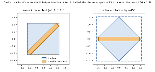
scripts/bg_certification_figures.py.In our chain. On the landing’s impact window, the zonotope’s hull was no tighter than a chain-rule enclosure over the first five steps, but its set was: its projection on (tilt, tilt rate) was smaller than its own hull by 0.27, 0.53, 0.79, 1.04 and 1.29 bits after steps 1 to 5. That kept correlation is what made the impact step’s reached set 14.5 bits (in volume) tighter than re-boxing.
3. Affine maps are exact
Intuition. A linear map sends each direction of uncertainty to a new direction. Nothing is lost.
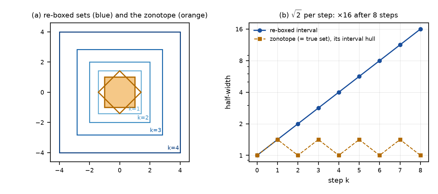
Check it by hand. Rotate the square \(\mathcal Z(0,I)\) by \(45^\circ\): the new generators are the columns of the rotation matrix, \((0.71,0.71)\) and \((-0.71,0.71)\), and the set is exactly the rotated square. After 8 rotations the generators are back to \(I\): no growth at all, where re-boxing grew 16-fold (interval arithmetic §3).
reports/technical-report/scripts/ch18_wrapping.py.The general statement. \[ A\,\mathcal Z(c,G)+b=\mathcal Z(Ac+b,\ AG),\qquad \mathcal Z(c_1,G_1)\oplus\mathcal Z(c_2,G_2)=\mathcal Z(c_1+c_2,\ [G_1,G_2]). \] Why: \(A(c+G\xi)+b=(Ac+b)+(AG)\xi\) for every \(\xi\), and stacking \((\xi_1,\xi_2)\) ranges over the bigger cube exactly when each part ranges over its own.
4. Affine arithmetic is zonotopes, one operation at a time
Intuition. Give every source of uncertainty a name, a noise symbol \(\epsilon_i\in[-1,1]\), and write every quantity as a centre plus multiples of the shared symbols. Then \(x-x\) cancels, because both copies carry the same symbol.
Check it by hand. \(x\in[1,2]\) becomes \(\hat x=1.5+0.5\,\epsilon_1\). Then \(\hat x-\hat x=0\), exactly: the dependency loss of interval arithmetic is gone. A product is not affine: \(\hat x\cdot\hat x=2.25+1.5\epsilon_1+0.25\epsilon_1^2\), and \(0.25\epsilon_1^2\in[0,0.25]\). Affine arithmetic keeps its midpoint, \(0.125\), and bounds the rest, \([-0.125,0.125]\), by a new symbol: \(\hat x^2=2.375+1.5\,\epsilon_1+0.125\,\epsilon_2\).
The general statement. A vector of affine forms over shared symbols is a zonotope [4]: centres form \(c\), coefficient columns form \(G\). Each nonlinear operation adds one generator for its error. The zonotope step below does the same for a whole step map at once.
5. Nonlinear steps: linear part plus a remainder
Intuition. Linearize the step at the centre, map the generators through the Jacobian exactly, and put whatever the linearization misses into a few extra generators.
Check it by hand. Let \(f(x)=x^2\) on \(\mathcal Z(1.5,[0.5])\), i.e. \(x\in[1,2]\). At the centre \(f(1.5)=2.25\) and \(f'(1.5)=3\), so the linear part is \(2.25+1.5\,\xi\). The second derivative is \(2\), so the Lagrange remainder is at most \(\tfrac12\cdot2\cdot0.5^2=0.25\). The result \(\mathcal Z(2.25,[1.5,\ 0.25])\) spans \([0.5,4]\) and contains the true range \([1,4]\).
The general statement. Let \(X=c+[-r,r]\) be the zonotope’s interval hull, \(r=|G|\mathbf 1\).
- Lagrange form: if \([H_j]\) bounds the Hessian of \(f_j\) on \(X\), \[ f(\mathcal Z(c,G))\subseteq\mathcal Z\big(f(c),\ [\,J_f(c)\,G,\ \operatorname{diag}(e)\,]\big), \qquad e_j=\tfrac12\,r^\top\big|[H_j]\big|\,r . \] The remainder is quadratic in the set’s size.
- Mean-value form: if \([J]\) bounds the Jacobian on \(X\) with midpoint \(M\) and radius \(\Delta\), \(f(\mathcal Z)\subseteq\mathcal Z(f(c),[MG,\ \operatorname{diag}(\Delta r)])\). The remainder is linear in \(r\) with coefficient \(\Delta\), and it carries every overestimate of the interval Jacobian; chained over steps, those multiply.
Why both are sound: Taylor’s theorem (Lagrange) or the mean value theorem, applied on the segment from \(c\) to any point of \(X\), which lies in the convex set \(X\).
6. Keeping the generator count bounded
Intuition. Each nonlinear step adds generators. Fold the smallest ones into a box: a small, controlled loss.
Check it by hand. \(\mathcal Z(0,[(1,1),(0.02,0.01),(0.01,-0.02)])\): box the last two generators. Their interval hull has half-widths \((0.03,0.03)\), so the reduced set is \(\mathcal Z(0,[(1,1),(0.03,0),(0,0.03)])\). It contains the original and is barely bigger.
The general statement. For \(G=[G_1,G_2]\), \(\mathcal Z(c,G)\subseteq\mathcal Z(c,[G_1,\operatorname{diag}(|G_2|\mathbf 1)])\), since \(\mathcal Z(0,G_2)\) lies in its own hull. Girard’s rule [2] boxes the generators that lose least when boxed. Our impact-window trees cap the count at 40; on the experiment’s sub-box the cap lost nothing in the hull against no cap, which reaches 307 generators by step 7.
7. Checking a condition: one line of arithmetic
Intuition. To find the smallest value of a linear quantity over a zonotope, push each \(\xi_i\) to whichever end hurts.
Check it by hand. On the thin zonotope of §1, the smallest \(x+y\) is \(0-|1+1|-|0.1-0.1|=-2\), and the smallest \(x-y\) is \(0-|1-1|-|0.1+0.1|=-0.2\).
The general statement. \[ \min_{x\in\mathcal Z(c,G)} a\cdot x \;=\; a\cdot c-\big\|G^\top a\big\|_1 \;=\; a\cdot c-\sum_i |a\cdot g_i| . \] A force floor, a friction cone edge or a motor limit is such a check, or its linearization plus a remainder: \(q(c)-\|G^\top\nabla q(c)\|_1-e\ge b\).
8. Containment: does one set lie inside another?
Intuition. Junctions between funnels ask whether one certified set lies inside the next (composition). Against a box this is exact; against a zonotope there is a quick sufficient test.
Check it by hand. Is the thin zonotope of §1 inside \([-1.2,1.2]^2\)? Its hull half-widths are \(|G|\mathbf 1=(1.1,1.1)\le1.2\): yes, exactly.
The general statement.
- Box outer: exact. \(\mathcal Z(c,G)\subseteq[l,u]\) iff \(c-|G|\mathbf 1\ge l\) and \(c+|G|\mathbf 1\le u\).
- Zonotope outer: a sufficient linear program. If \(G_1=G_2\Gamma\), \(c_1-c_2=G_2\beta\) and every row of \([\Gamma,\beta]\) has absolute sum \(\le1\), then \(\mathcal Z(c_1,G_1)\subseteq\mathcal Z(c_2,G_2)\) [5], because \(c_1+G_1\xi=c_2+G_2(\beta+\Gamma\xi)\). The LP’s answer is re-verified exactly before it counts. Exact zonotope containment is hard in general, so a “no” from the LP does not prove non-containment.
9. Branches at a contact switch
Intuition. At an impact, part of the set makes contact and part does not, and each part follows its own contact mode. A zonotope cut by a half-space is no longer a zonotope.
The general statement. A constrained zonotope \(\{c+G\xi:\ \xi\in[-1,1]^m,\ A\xi=b\}\) is closed under such cuts [6]. A hybrid zonotope adds binary factors \(\xi^b\in\{-1,1\}^{n_b}\): a union of \(2^{n_b}\) constrained zonotopes sharing generators, one per mode branch. Checks on them are linear programs per branch [7]. This is the foundation we build on: Bird, Pangborn, Jain and Koeln, Automatica 2023, Siefert et al., ACC 2023, functional decomposition and the zonoLAB toolbox.
In our chain. The impact window’s census found the binding step to be the tail after the make, where the disk may slide during the impact. That is wrapping in the data, not branching, so hybrid zonotopes would not help there; tighter enclosures would.
10. What the records show
- First experiment (chain-rule Jacobians intersected with the box): the make step’s reached set \(2^{8.8}\)–\(2^{12.6}\) times tighter in volume, the tail alone looser; the boxes on which post-impact rocking is excluded grew \(2^{12}\) in volume. That number is an exclusion-box gain, not a reached-set shrinkage.
- Zonotope tree, day-1 census over the whole impact window: every one of 64 probe cells certifies; the projected cover is \(2.7\times10^7\) pieces (95% band \(1.9\)–\(3.6\times10^7\)) against about \(2^{36}\) re-boxed.
- The cover itself is running on the current landing set (status in
reports/supporting_docs/landing_motion/zonotope-cover-status.typ).
What to remember
- A zonotope is a centre plus generators; a box is the diagonal case.
- Affine maps are exact: no re-boxing, no wrapping.
- A nonlinear step is linear part plus remainder generators (Lagrange: quadratic; mean-value: linear, inheriting the Jacobian’s overestimate).
- Same hull is not the same set: the hidden correlation pays off at later steps.
- Checks are closed form, \(a\cdot c-\|G^\top a\|_1\); containment in a box is exact, in a zonotope a sufficient LP whose answer is re-verified.
- Mode branches use constrained and hybrid zonotopes (Koeln et al.).
Further reading
- Girard [2]: the clearest short introduction to zonotope reachability, including order reduction; start here.
- Kühn [1]: zonotopes as the cure for the wrapping effect in rigorous orbit computation.
- Nedialkov, Jackson and Corliss [3]: survey of validated ODE integration, with Lohner’s parallelepiped (QR) method.
- de Figueiredo and Stolfi [4]: affine arithmetic, the operation-by-operation view of zonotopes.
- Scott, Raimondo, Marseglia and Braatz [6]: constrained zonotopes, exact intersections at the cost of linear programs.
- Bird, Pangborn, Jain and Koeln [7] and Siefert et al. [8]: hybrid zonotopes for mode-branched sets and their nonlinear successor sets, the foundation we build on; the zonoLAB toolbox [9] implements them.
- Althoff’s CORA [10] and Kochdumper and Althoff’s sparse polynomial zonotopes [11]: a mature zonotope reachability toolbox, and the higher-order set that keeps nonlinear correlations.
- Berz and Makino [12]: Taylor models, polynomial enclosures with interval remainders, the higher-order relative of the first-order zonotope step.
- Sadraddini and Tedrake [5]: linear encodings of polytope and zonotope containment.