Background: control barrier functions
Safety as an invariant set: what a barrier function proves and why, how it relates to a Lyapunov function, how a control barrier function becomes a safety filter on a nominal controller, a block pushed toward a wall by hand, the extensions that matter for contact, and where barrier conditions already sit in our certificates.
Before this page: interval arithmetic, zonotopes and certified funnels and composition. Its companion is dissipation (passivity) certificates: a storage function bounds an energy from above, a barrier function bounds a margin from below. The terminology: the block is the manipulated object; a box is only an interval box (a product of intervals).
Who this is for. You know state-space control and Lyapunov functions. This page builds control barrier functions (CBFs) from one idea, proves the results it uses, relates them to Lyapunov functions, works one example by hand, and ends with a reading list.
1. Safety as set invariance
Intuition. “Safe” usually means “never leaves a region”: the block never reaches the wall, a normal force never drops below a floor, a tilt never exceeds a bound. Write the region as the set where a scalar margin is nonnegative. Safety then says: a motion that starts with a nonnegative margin keeps it nonnegative forever.
The setting. Take a system \(\dot x=f(x)\) with state \(x\in\mathbb R^n\), and a continuously differentiable function \(h:\mathbb R^n\to\mathbb R\). The safe set is
\[ C=\{x:\ h(x)\ge 0\},\qquad \partial C=\{x:\ h(x)=0\},\qquad \operatorname{Int}C=\{x:\ h(x)>0\}. \tag{1}\]
The last two equalities need \(\nabla h\neq0\) where \(h=0\); Example 5 shows what goes wrong without it.
Definition 1 (Forward invariance) In plain words: every motion that starts in \(C\) stays in \(C\). Formally, \(C\) is forward invariant if for every \(x_0\in C\) the solution with \(x(0)=x_0\) satisfies \(x(t)\in C\) for all \(t\ge0\) for which it exists.
Example 1 (Invariant or not) Let \(h(x)=1-x^2\), so \(C=[-1,1]\). With \(\dot x=-x\), every motion decays toward 0 and never leaves \([-1,1]\): \(C\) is forward invariant. With \(\dot x=+x\), the motion from \(x_0=0.5\) reaches \(x=1\) at \(t=\ln2\) and leaves: not invariant.
Nagumo’s theorem is the exact test, and it looks only at the boundary.
Theorem 1 (Nagumo [1], [2]) Suppose \(\dot x=f(x)\) has a unique solution from every initial state. A closed set \(C\) is forward invariant if and only if \(f(x)\in T_C(x)\) at every \(x\in\partial C\).
Here \(T_C(x)\) is the (Bouligand) tangent cone: the directions \(d\) with \(\liminf_{\tau\downarrow0}\operatorname{dist}(x+\tau d,C)/\tau=0\), that is, the directions in which one can move from \(x\) while leaving \(C\) by less than first order. If \(h\) is continuously differentiable and \(\nabla h(x)\neq0\), then \(T_C(x)=\{d:\nabla h(x)\cdot d\ge0\}\), and the test reads
\[ \dot h(x)=\nabla h(x)\cdot f(x)\;\ge\;0\qquad\text{for every }x\in\partial C . \tag{2}\]
Uniqueness matters: without it, the tangent condition guarantees only that some solution stays in \(C\).
2. From barrier certificates to control barrier functions
Barrier certificates: verification, no input
Prajna and Jadbabaie [3] asked a verification question: given \(\dot x=f(x,d)\) with a disturbance \(d\), an initial set \(X_0\) and an unsafe set \(X_u\), can any motion get from \(X_0\) to \(X_u\)? A barrier certificate is a function \(B\) with
\[ B(x)\le0\ \text{on } X_0,\qquad B(x)>0\ \text{on } X_u,\qquad \nabla B(x)\cdot f(x,d)\le0\ \text{for all } x,d . \tag{3}\]
\(B\) never increases, so it can never climb from \(\le0\) to \(>0\): no motion from \(X_0\) reaches \(X_u\). With \(h=-B\) this is “\(\dot h\ge0\) everywhere”, Proposition 1. They searched for \(B\) by sums-of-squares programming, and the journal version adds a stochastic certificate (a supermartingale) [4]. There is no input: the controller, if any, is already inside \(f\).
Control barrier functions: synthesis, with an input
With a control-affine system
\[ \dot x=f(x)+g(x)\,u,\qquad u\in U\subseteq\mathbb R^m , \tag{4}\]
the derivative of \(h\) depends on the input: \(\dot h=L_fh(x)+L_gh(x)\,u\), with the Lie derivatives \(L_fh=\nabla h\cdot f\) (a scalar) and \(L_gh=\nabla h\cdot g\) (a row of \(m\) numbers). The question changes from “is the system safe?” to “is there an input that keeps it safe?”. Wieland and Allgöwer first proposed the control barrier function [5], by analogy with the control Lyapunov function; Ames, Grizzle and Tabuada turned it into the quadratic program used today [6], [7].
Definition 2 (Extended class-\(\mathcal K\) function) In plain words: a continuous, strictly increasing function through the origin that is also defined for negative arguments. Formally, \(\alpha:(-b,a)\to\mathbb R\) with \(a,b>0\), continuous, strictly increasing, and \(\alpha(0)=0\). The everyday choice is \(\alpha(h)=\gamma h\) with \(\gamma>0\).
Definition 3 (Zeroing control barrier function [7], [8]) Let \(h\) be continuously differentiable, \(C=\{h\ge0\}\), and \(D\supseteq C\) an open set. \(h\) is a control barrier function on \(D\) if there is an extended class-\(\mathcal K\) function \(\alpha\) such that
\[ \sup_{u\in U}\big[\,L_fh(x)+L_gh(x)\,u\,\big]\;\ge\;-\alpha\big(h(x)\big)\qquad\text{for every } x\in D . \tag{5}\]
The admissible inputs at \(x\) form \[ K_{\rm cbf}(x)=\{u\in U:\ L_fh(x)+L_gh(x)u\ge-\alpha(h(x))\}. \]
The claim, proved as Proposition 2: any locally Lipschitz feedback \(u(x)\in K_{\rm cbf}(x)\) keeps \(C\) forward invariant.
Read the condition. Inside \(C\), \(h>0\) and \(\alpha(h)>0\), so \(h\) may decrease, but no faster than \(\alpha(h)\). On the boundary, \(\alpha(0)=0\), so \(\dot h\ge0\), which is Nagumo’s condition Equation 2. Outside \(C\), \(\alpha(h)<0\), so \(h\) must increase: the state is pushed back.
Why the \(\alpha(h)\) form. The earlier conditions were “\(\dot h\ge0\) everywhere” (barrier certificates) or its reciprocal analogue, and Ames et al. note both are too restrictive in the interior of \(C\) [7]: they freeze every level set of \(h\), so a controller may never spend margin, even far from the boundary. Two forms relax this.
- The reciprocal form uses \(B=1/h\), which blows up at the boundary, with a condition like \(\dot B\le\gamma/B\) [6]. \(B\) is not defined outside \(C\), and the constraint becomes ill-conditioned near \(\partial C\).
- The zeroing form Equation 5 is defined on an open \(D\) that reaches outside \(C\). It makes \(C\) asymptotically stable as well as invariant, and that is the source of its robustness: a small disturbance that pushes the state out is pushed back [7], [9]. It is the form used almost everywhere now, and on the rest of this page.
3. Why it works: the invariance proofs
Standing assumptions. Every result below uses these.
- The system. \(\dot x=f(x)\) with \(f\) locally Lipschitz. For the CBF case, \(f\) is the closed loop \(f(x)+g(x)u(x)\), and the feedback \(u(x)\) is locally Lipschitz too (Remark 2 below says when the CBF-QP’s feedback is).
- Unique solutions. Local Lipschitz continuity gives, for each \(x_0\), a unique solution \(x(t)\) on a maximal interval \([0,T)\). “For all \(t\)” below means all \(t\in[0,T)\); whether \(T=\infty\) is a separate question.
- The margin. \(h\) is continuously differentiable, and \(\dot h(x):=\nabla h(x)\cdot f(x)\). Along a solution, the chain rule makes \(m(t)=h(x(t))\) continuously differentiable, with \(\dot m(t)=\dot h(x(t))\).
Two tools.
Definition 4 (First exit time) In plain words: the last moment up to which a motion has stayed in \(C\) the whole time. Formally, \[ t^*=\sup\{\tau\in[0,T):\ x(s)\in C\text{ for all } s\in[0,\tau]\}. \] If \(C\) is not forward invariant, some motion from \(C\) has \(t^*<T\), and there are times just after \(t^*\) at which it is outside \(C\).
Lemma 1 (Comparison lemma) In plain words: if a quantity always grows at least as fast as the solution of a reference scalar equation would at the same value, and starts no lower, it stays no lower. Formally, let \(\dot y=\varphi(y)\) with \(\varphi\) locally Lipschitz have the solution \(y(t)\) on \([0,T_1)\). If a continuously differentiable \(m\) satisfies \(\dot m(t)\ge\varphi(m(t))\) and \(m(0)\ge y(0)\), then \(m(t)\ge y(t)\) on \([0,T_1)\). This is Khalil’s Lemma 3.4 [10], stated there for upper bounds and applied here to \(-m\).
The margin never decreases
Proposition 1 (Barrier certificate) Let \(D\) be an open set containing \(C\). If \(\dot h(x)\ge0\) for every \(x\in D\), then \(C\) is forward invariant.
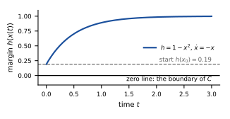
Intuition. The margin can never shrink, so it can never fall from \(\ge0\) to \(<0\).
Proof. Take \(x_0\in C\) and suppose, for a contradiction, that the motion leaves \(C\).
- First exit time. Then \(t^*<T\), and every interval \((t^*,t^*+\delta)\) contains times at which \(x(t)\notin C\).
- Continuity, and \(C\) closed. \(x(t)\in C\) for \(t<t^*\), \(x\) is continuous, and \(C=\{h\ge0\}\) is closed because \(h\) is continuous. So \(x(t^*)\in C\).
- \(D\) open, continuity. \(x(t^*)\in C\subseteq D\) and \(D\) is open, so for some \(\varepsilon>0\), \(x(t)\in D\) for all \(t\in[0,t^*+\varepsilon)\).
- Monotonicity. On that interval \(\dot m(t)=\dot h(x(t))\ge0\), so \(m(t)\ge m(0)=h(x_0)\ge0\): \(x(t)\in C\) on \([0,t^*+\varepsilon)\).
- Contradiction. Step 4 contradicts step 1 with \(\delta=\varepsilon\).
This is a Lyapunov argument: \(V=-h\) never increases, so its sublevel set \(\{V\le0\}=C\) is invariant, exactly as the sublevel sets of a Lyapunov function are (§4 makes this precise). Step 3 is why the condition must hold on an open \(D\) and not only on \(C\); Example 5 shows that the step cannot be skipped.
Example 2 (Check Proposition 1 by hand) \(\dot x=-x\) and \(h=1-x^2\) give \(\dot h=-2x\dot x=2x^2\ge0\) on all of \(\mathbb R\). From \(x_0=0.9\), \(h(x_0)=0.19\). At \(t=1\), \(x=0.9e^{-1}=0.331\) and \(h=1-0.81e^{-2}=0.890\ge0.19\).
The margin may shrink, but not past zero
Proposition 2 (Zeroing barrier function) Let \(\alpha\) be extended class-\(\mathcal K\) and locally Lipschitz, and \(D\) an open set containing \(C\). If \(\dot h(x)\ge-\alpha(h(x))\) for every \(x\in D\), then \(C\) is forward invariant. For the closed loop \(f+gu(x)\), this proves that a locally Lipschitz \(u(x)\in K_{\rm cbf}(x)\) keeps \(C\) safe.
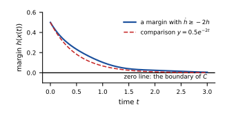
Intuition. \(h\) is a distance-like margin to the unsafe set. The condition says the margin may shrink, but never faster than \(\alpha(h)\), and \(\alpha(0)=0\) means it stops shrinking exactly at the boundary.
Proof. Take \(x_0\in C\).
- The comparison system. Let \(y(t)\) solve \(\dot y=-\alpha(y)\) with \(y(0)=h(x_0)\ge0\).
- Uniqueness: zero is a floor. Since \(\alpha(0)=0\), the constant \(y\equiv0\) is a solution. \(\alpha\) is locally Lipschitz, so solutions are unique, and two different solutions can never meet. So if \(y(0)>0\), then \(y(t)>0\) for all \(t\), and if \(y(0)=0\), then \(y\equiv0\). Either way \(y(t)\ge0\). It exists for all \(t\ge0\): while \(y>0\), \(\dot y<0\), so \(y\) stays in \([0,y(0)]\).
- First exit time, \(D\) open. Suppose the motion leaves \(C\). As in steps 1–3 of the proof of Proposition 1, \(t^*<T\), \(x(t^*)\in C\), and \(x(t)\in D\) on \([0,t^*+\varepsilon)\).
- Comparison. On that interval, \(\dot m\ge-\alpha(m)\) and \(m(0)=y(0)\), so Lemma 1 with \(\varphi=-\alpha\) gives \(m(t)\ge y(t)\ge0\).
- Contradiction. So \(x(t)\in C\) on \([0,t^*+\varepsilon)\), against the definition of \(t^*\).
Remark 1 (where the condition bites). In the interior, \(\alpha(h)>0\), so the condition allows \(\dot h<0\): the controller may spend margin. Only at the boundary does it demand \(\dot h\ge0\). This is what makes the zeroing form less restrictive than Proposition 1.
Remark 2 (the feedback must be Lipschitz). The proof needs unique closed-loop solutions. Suppose \(f\), \(g\), \(\nabla h\), \(\alpha\) and the nominal controller are locally Lipschitz, and \(L_gh(x)\neq0\). Then the single-constraint CBF-QP of §5 has the closed form Equation 11. It is built from Lipschitz operations (\(\max(0,\cdot)\), products, and division by \(\lVert L_gh\rVert^2\) away from zero), so its feedback is locally Lipschitz. Ames et al. prove the same for the QP that combines a CBF with a control Lyapunov function, under this relative-degree-one condition [7], Thm. 3. They also note that once input bounds are added as further QP constraints, Lipschitz continuity is no longer assured.
Example 3 (Check Proposition 2 by hand) With \(\alpha(h)=2h\) and \(h(x_0)=0.5\), the bound is \(h(t)\ge0.5e^{-2t}\). That is \(0.068\) at \(t=1\) and \(0.0012\) at \(t=3\): shrinking, never negative. The bound reaches zero only as \(t\to\infty\), so a filtered motion approaches the boundary without touching it in finite time. Run B of Example 8 shows this.
Discrete time: the form a time-stepped certifier uses
Proposition 3 (Discrete-time barrier function) Let \(x_{k+1}=F(x_k)\), and \(\gamma\in(0,1]\). If
\[ h(F(x))-h(x)\;\ge\;-\gamma\,h(x)\qquad\text{for every }x\in C, \tag{6}\]
then from any \(x_0\in C\), \(h(x_k)\ge(1-\gamma)^k\,h(x_0)\ge0\) for all \(k\ge0\).
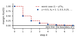
Intuition. Each step may spend at most the fraction \(\gamma\) of the margin it has, and spending a fraction of something nonnegative leaves something nonnegative.
Proof.
- Rearrange. At \(x_k\in C\), Equation 6 reads \(h(x_{k+1})\ge(1-\gamma)\,h(x_k)\).
- Induction, base. \(h(x_0)=(1-\gamma)^0h(x_0)\) and \(h(x_0)\ge0\).
- Induction, step. If \(h(x_k)\ge(1-\gamma)^kh(x_0)\ge0\), then \(x_k\in C\), so step 1 applies. Since \(1-\gamma\ge0\), \[ h(x_{k+1})\ge(1-\gamma)h(x_k)\ge(1-\gamma)^{k+1}h(x_0)\ge0. \]
Nothing in the proof needs continuity, differentiability or Lipschitz constants. \(F\) may be a simulator step or a step with an impact in it, and \(h\) may have kinks. Nor does the condition need an open \(D\): a step lands where it lands, and Equation 6 at \(x_k\) bounds \(h\) there directly. This is Agrawal and Sreenath’s discrete-time CBF [11]. With an input, \(F(x,u)\), the condition is a constraint on \(u\), but in general no longer an affine one (§7).
Example 4 (Check Proposition 3 by hand) \(\gamma=0.5\), \(h_0=1\): the bound is \(1, 0.5, 0.25, 0.125,\dots\), never negative. If \(\gamma>1\) were allowed, say \(\gamma=1.5\), the bound would read \(1,-0.5,\dots\): unsafe after one step. That is why \(\gamma\le1\). With \(\gamma=1\), the condition is just “the next state is safe”.
A counterexample: why the boundary-only condition needs care
Example 5 (The gradient test can be fooled) Let \(h(x)=-x^2\), so \(C=\{0\}\), and \(\dot x=1\). Then \(\dot h\ge0\) at every point of \(C\), yet the motion from \(x_0=0\) leaves \(C\) at once.
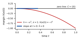
Why the intuition breaks. The margin \(h=-x^2\) has zero slope at the boundary, so “\(\dot h\ge0\) at the boundary” says nothing there.
- The condition holds on \(C\). \(\dot h=-2x\cdot1=-2x\), which is \(0\ge0\) at \(x=0\), the only point of \(C\).
- The motion leaves. \(x(t)=t\), so \(h(x(t))=-t^2<0\) for every \(t>0\).
- What failed. \(\nabla h(0)=0\). Proposition 1 asks for \(\dot h\ge0\) on an open \(D\ni0\), and that fails: at any \(x>0\), \(\dot h=-2x<0\). Step 3 of its proof is the step this example breaks.
- What Nagumo says. A single point’s tangent cone is \(T_C(0)=\{0\}\), and \(f=1\notin T_C(0)\), so Theorem 1 correctly says “not invariant”. The gradient form Equation 2 is only valid where \(\nabla h\neq0\).
With a bounded disturbance
Proposition 4 (Robust margin, input-to-state safety) Let \(\dot x=f(x)+g(x)u+p(x)w\) with \(\lVert w(t)\rVert\le\bar w\), and \(c=\sup_{x\in D}\lVert\nabla h(x)\,p(x)\rVert\). Suppose the feedback meets the nominal condition \(L_fh+L_ghu\ge-\gamma h\) on \(D\). Then every disturbed motion has \(\dot h\ge-\gamma h-c\bar w\), and the slightly inflated set \(C_w=\{h\ge-c\bar w/\gamma\}\) is forward invariant (when \(C_w\subseteq D\)).
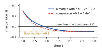
Intuition. The disturbance can steal at most \(c\bar w\) of margin per unit time, and the barrier condition restores \(\gamma h\), so the two balance at \(h=-c\bar w/\gamma\).
Proof. \(\tilde h=h+c\bar w/\gamma\) satisfies \(\dot{\tilde h}=\dot h\ge-\gamma\tilde h\), so Proposition 2 applies to \(\tilde h\). Its proof uses only this inequality along the motion, so a time-varying \(w(t)\) is fine.
To keep \(C\) itself, demand the margin up front: \(L_fh+L_ghu\ge-\gamma h+c\bar w\). For general \(\alpha\), and for choosing the margin as a function of \(L_gh\), see input-to-state safety [12] and the robustness of zeroing CBFs [9], [13]; this page states the linear case only.
Example 6 (Check Proposition 4 by hand) \(\gamma=2\), \(c\bar w=0.2\): the floor is \(-0.1\). A motion with \(h(0)=0.3\) satisfies \(h(t)\ge-0.1+0.4e^{-2t}\).
4. Lyapunov functions and barrier functions: the same idea, two jobs
The question. A Lyapunov function has \(\dot V\le0\); a barrier function has \(\dot h\ge0\). One decreases, the other increases. How do the two fit?
The sign is only a convention
| Lyapunov | Barrier | |
|---|---|---|
| Good region | a sublevel set \(\{V\le c\}\) | a superlevel set \(\{h\ge0\}\) |
| Condition | \(\dot V\le0\) | \(\dot h\ge0\), or \(\dot h\ge-\alpha(h)\) |
| In words | \(V\) never climbs toward the edge | \(h\) never falls toward the edge |
The sign says which side of a level set is good. Flip it:
\[ h=c-V\qquad\Longrightarrow\qquad \dot h=-\dot V, \tag{7}\]
and “\(\dot V\le0\)” becomes “\(\dot h\ge0\)”. Both say the same thing: the scalar never moves toward the boundary of the good set.
Lyapunov gives barriers for free
Proposition 5 (Lyapunov gives barriers for free) Let \(V\) be continuously differentiable with \(\dot V(x)=\nabla V(x)\cdot f(x)\le0\) for every \(x\in\mathbb R^n\). Then every sublevel set \(\{V\le c\}\) is forward invariant.
Proof. Fix \(c\) and let \(h_c=c-V\). Then \(\{h_c\ge0\}=\{V\le c\}\), and by Equation 7, \(\dot h_c=-\dot V\ge0\) on \(\mathbb R^n\), which is an open set containing \(\{h_c\ge0\}\). Proposition 1 applies.
One Lyapunov function hands you a whole nested family of safe sets, one per level \(c\). The proof never used \(V\ge0\) or an equilibrium; those matter for convergence, not for invariance.
The converse fails
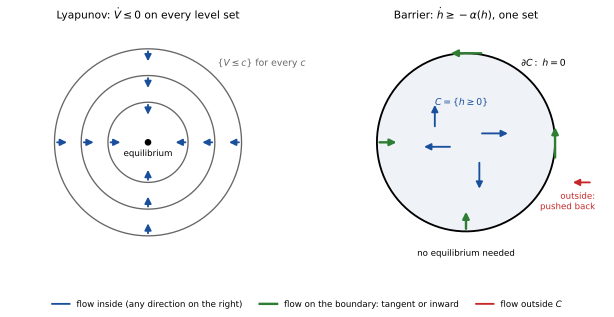
scripts/bg_cbf_figures.py.A barrier function does not give a Lyapunov function back.
- One set, no convergence. A barrier certifies one set, and says nothing about where motions go inside it.
- No equilibrium. The set need not contain an equilibrium at all, and \(h\) is sign-indefinite: positive inside, negative outside.
- Binding only at the boundary. The CBF condition Equation 5 lets \(h\) decrease inside \(C\) (the state may drift toward the boundary) and forces \(\dot h\ge0\) only where \(h=0\), because \(\alpha(0)=0\).
In Lyapunov form, with \(h=c-V\), the zeroing condition reads
\[ \dot V\;\le\;\alpha\big(c-V\big). \tag{8}\]
This is the Lyapunov condition, relaxed in the interior (\(V<c\) allows \(\dot V>0\)) and enforced on the level set \(\{V=c\}\).
Side by side
| Control Lyapunov function (CLF) | Control barrier function (CBF) | |
|---|---|---|
| Certifies | stability: convergence to an equilibrium or a set | safety: forward invariance of one set |
| Sign | \(V\ge0\), positive definite about the target | \(h\) sign-indefinite: \(\ge0\) on \(C\), \(<0\) outside |
| Holds on | everywhere in the region of interest | an open neighbourhood of \(C\); binding at \(\partial C\) |
| Equilibrium needed | yes | no |
| Strict form | \(\dot V\le-\alpha(V)\) | \(\dot h\ge-\alpha(h)\) |
| Control version | \(\inf_u\big[L_fV+L_gVu\big]\le-\alpha(V)\) | \(\sup_u\big[L_fh+L_ghu\big]\ge-\alpha(h)\) |
| Discrete time | \(V(x_{k+1})\le V(x_k)\) | \(h(x_{k+1})\ge(1-\gamma)h(x_k)\) |
| Converse theorem | asymptotic stability implies a Lyapunov function exists [10], [14] | safety implies a barrier certificate exists, under conditions on the flow [15], [16] |
| Verification | sums of squares, LP, or set-based enclosures | the same: sums of squares, LP, or set-based enclosures |
| In the CLF–CBF QP | a soft constraint, with a slack | a hard constraint |
: CLF and CBF side by side {#tbl-clf-cbf}
The converse theorems. For Lyapunov functions, Massera proved that asymptotic stability implies the existence of a Lyapunov function [14]; Khalil’s §4.7 collects the converse theorems [10]. For barrier certificates, Prajna and Rantzer proved necessity for flows with neither singular points nor closed orbits [15]. Wisniewski and Sloth extended it to a class of structurally stable systems with several singular elements, after redefining safety to suit them [16]. Safety alone is not enough: the flow must be regular enough.
The CLF–CBF quadratic program [7]. Both conditions are affine in \(u\), so one QP can carry both:
\[ \begin{aligned} \min_{u,\,\delta}\quad & \tfrac12\lVert u-u_{\rm ref}\rVert^2+p\,\delta^2\\ \text{s.t.}\quad & L_fV+L_gV\,u\le-\alpha_V(V)+\delta &&\text{(stability, soft)}\\ & L_fh+L_gh\,u\ge-\alpha(h) &&\text{(safety, hard)} \end{aligned} \tag{9}\]
Stability is a soft constraint: the slack \(\delta\), penalized by \(p>0\), lets it give way. Safety is hard. The order follows the stakes: when the two conflict (the target lies beyond an obstacle), the controller should give up progress, not safety. The slack also keeps the QP feasible whenever the CBF constraint alone is (with \(L_gh\neq0\)). Ames et al.’s Lipschitz result is stated for this relaxed form [7], Thm. 3.
What it means for this project
The storage function \(S\) of the dissipation certificates is Lyapunov-like with a supply: \(\dot S\le s-d\). With zero supply, it is a Lyapunov function. Its sublevel sets are barrier sets through \(h=c-S\) (Proposition 5). So storage and barrier are two jobs of one idea: the first proves that the block comes to rest, the second proves where it can never go.
Example 7 (The tilt: a bound, not a decrease) Take the tilt margin \(h=\theta_{\max}-\theta\). A tilt barrier needs only that the tilt never crosses its bound; it does not need the tilt to shrink. During a support switch, the block may rock slightly, so the tilt grows a little. A Lyapunov-style “the tilt decreases everywhere” would be false there. The barrier condition \(\dot h\ge-\alpha(h)\) still allows that growth while margin remains, and binds only at \(\theta=\theta_{\max}\). This illustrates the idea; no result is claimed here.
5. The CBF-QP safety filter
Intuition. Keep a controller you already trust for performance (the nominal one), and change its output only when safety requires it, and then as little as possible.
The precise statement [6], [7]. At each state \(x\), apply
\[ u^*(x)=\arg\min_{u\in U}\ \tfrac12\lVert u-u_{\rm nom}(x)\rVert^2 \quad\text{s.t.}\quad L_fh(x)+L_gh(x)\,u+\alpha(h(x))\ge0 . \tag{10}\]
The constraint is affine in \(u\), so with a polyhedral \(U\) this is a quadratic program: small, convex, and fast enough to solve at every control step.
One constraint, no input bounds: a closed form. Write \(\psi(x)=L_fh+L_gh\,u_{\rm nom}+\alpha(h)\), the slack the nominal input leaves. If \(\psi\ge0\), the nominal input is already safe, and \(u^*=u_{\rm nom}\). Otherwise, project onto the constraint’s half-space:
\[ u^*=u_{\rm nom}+\frac{\max\big(0,\,-\psi(x)\big)}{\lVert L_gh(x)\rVert^2}\,L_gh(x)^{\top}\qquad(L_gh\neq0). \tag{11}\]
The filter is inactive far from the boundary, and it pushes only along \(L_gh^\top\), the input direction that changes \(h\) fastest.
Feasibility.
- No input bounds. With \(U=\mathbb R^m\) and \(L_gh(x)\neq0\), the constraint can always be met. Where \(L_gh(x)=0\), it is a condition on the state alone, and the QP is infeasible whenever it fails. That is the relative-degree problem of Example 8.
- Input bounds. With bounded \(U\), the “\(\sup_{u\in U}\)” in Equation 5 is the whole difficulty. A function that is a CBF for unbounded inputs may not be one for \(\lVert u\rVert\le u_{\max}\): near the boundary, no admissible input can stop the decrease, and the QP becomes infeasible. Valid CBFs under input bounds must build the braking ability into \(h\) [7], [17]. Run C of Example 8 shows it.
- Several constraints. Each may be satisfiable alone but not jointly, and the QP’s Lipschitz continuity is then not assured [7].
6. A worked toy: a block pushed toward a wall
Example 8 (A block pushed toward a wall) A block slides without friction on a line, at position \(x\) and speed \(v\). It is driven by an acceleration \(u\), and a wall stands at \(x_{\max}=100\) mm. The nominal controller pushes it toward the wall with \(u_{\rm nom}=0.5\) m/s². Safety: \(h=x_{\max}-x\ge0\), with \(\dot x=v\), \(\dot v=u\).
The first try fails: relative degree 2. \(\dot h=-v\) contains no \(u\): \(L_gh=0\). The CBF condition \(-v\ge-\gamma h\) is a condition on the state, which the input cannot enforce at this instant. The input reaches \(h\) only through \(\ddot h=-u\); \(h\) has relative degree 2.
The fix: an exponential (high-order) CBF [18], [19]. Make the barrier condition itself the new margin,
\[ h_1=\dot h+\lambda h=-v+\lambda(x_{\max}-x), \tag{12}\]
and impose a first-order CBF condition on \(h_1\), which does contain \(u\):
\[ \dot h_1+\lambda h_1\ge0\iff -u-\lambda v+\lambda(-v+\lambda h)\ge0 \iff u\le\lambda^2h-2\lambda v . \tag{13}\]
By Proposition 2, \(h_1\ge0\) is kept. And \(h_1\ge0\) means \(\dot h\ge-\lambda h\), so Proposition 2 again keeps \(h\ge0\). The invariant set is \(C\cap\{h_1\ge0\}\): closer to the wall, the block must be slower, \(v\le\lambda(x_{\max}-x)\). Here the closed form Equation 11 is simply \(u^*=\min\big(u_{\rm nom},\ \lambda^2h-2\lambda v\big)\).
With numbers (\(\lambda=5\) s⁻¹, so \(u\le 25h-10v\)):
- A, no filter, from \(v_0=100\) mm/s. The block hits the wall at \(v=\sqrt{0.1^2+2(0.5)(0.1)}=332\) mm/s, at \(t=(0.332-0.1)/0.5=463\) ms.
- B, filtered, from \(v_0=100\) mm/s. At the start, \(25(0.1)-10(0.1)=1.5>0.5\), so the filter is inactive. It switches on at \(x=15.8\) mm, \(v=161\) mm/s, where \(25h-10v\) drops to \(0.5\). It then brakes, at most \(0.327\) m/s², and the block creeps toward the wall: \(98.3\) mm after \(1.2\) s, never reaching it.
- C, filtered, with braking limited to \(|u|\le a_{\max}=1\) m/s², from \(v_0=480\) mm/s. The start satisfies \(h_1=-0.48+0.5=0.02\ge0\), but the filter asks for \(u=2.5-4.8=-2.3\) m/s² at once. That is beyond the limit, so the QP is infeasible, and saturated braking hits the wall at \(\sqrt{0.48^2-2(1)(0.1)}=174\) mm/s.
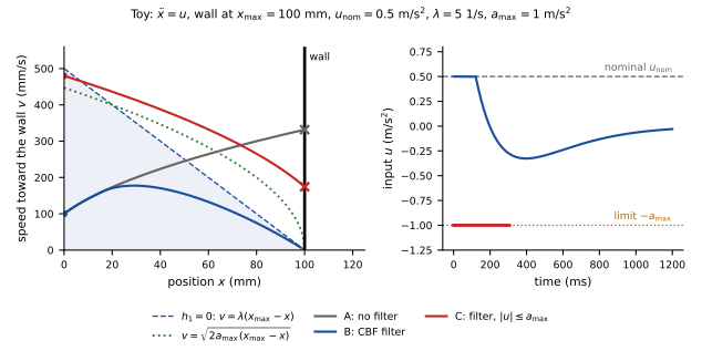
scripts/bg_cbf_figures.py.What C teaches. From \(v_0=480\) mm/s, the shortest stopping distance is \(v_0^2/(2a_{\max})=115.2\) mm \(>100\) mm. No admissible input saves the block, so \(h_1\) is not a valid CBF for \(|u|\le1\): its “\(\sup_{u\in U}\)” fails near the wall at high speed. A barrier that knows the limit is the braking margin
\[ h_b=x_{\max}-x-\frac{v\,|v|}{2a_{\max}},\qquad \dot h_b=-v-\frac{|v|}{a_{\max}}\,u , \tag{14}\]
which is continuously differentiable. For \(v>0\), full braking \(u=-a_{\max}\) gives \(\dot h_b=0\ge-\alpha(h_b)\), so the condition can always be met within the limit. Its zero set is the green curve. The same idea, a braking distance inside \(h\), is the adaptive-cruise-control barrier of [6], [7]. A good choice of \(h\) can remove both the relative-degree problem (\(L_gh_b\neq0\) for \(v\neq0\)) and the input-bound problem. Making that choice is the hard part.
7. Practical extensions
Each item gives the problem and its key references.
- High relative degree. Exponential CBFs stack the derivatives \(h,\dot h,\dots,h^{(r-1)}\) and place real poles by linear-system design [18]. High-order CBFs chain class-\(\mathcal K\) functions, \(\psi_i=\dot\psi_{i-1}+\alpha_i(\psi_{i-1})\), as Equation 12 did [19], [20]. Input bounds with high relative degree are treated in [17], and mechanical systems with torque inputs and position limits in [21].
- Disturbances and model error. The zeroing form is robust: \(C\) is asymptotically stable, so a perturbation only inflates it [9]. Robust CBFs add worst-case margins [13]. Input-to-state safety bounds the inflation by a class-\(\mathcal K\) function of the disturbance’s size [12], as in Proposition 4.
- Discrete time and sampling. The step condition Equation 6 is generally not affine in \(u\), so the filter becomes a nonlinear program (a quadratically constrained QP under conditions). It also sits naturally in model predictive control [22]. A continuous-time CBF applied with a zero-order hold needs a margin for the drift between samples [23]. Verifying a candidate discrete-time CBF over a set is a branch-and-bound global optimization [24].
- Nonsmooth and hybrid. The max and min of several barriers (Boolean combinations) give nonsmooth barriers on differential inclusions [25]. For hybrid systems with flows and jumps (an impact is a jump), sufficient conditions pair a flow condition with a jump condition [26]. Walking robots are the classic example of CBFs across impacts [27], [28].
- Stochastic. With noise, invariance holds with a probability, through a supermartingale condition [4]. CBFs for stochastic differential equations are developed in [29].
- Learned and neural CBFs, and their verification. For a survey, see [30]. A learned \(h\) is only a candidate until verified over the whole set. Verification can be exact over a ReLU network’s linear pieces [31], use bound propagation with branch and bound inside training [32], or, for parametric barriers, use interval analysis [33]. Hamilton–Jacobi reachability can refine or construct CBFs [34], [35].
- Set-based safety filters. Zonotopic safe sets with safety-preserving controllers for sampled-data systems [36]; a set-based CBF built from a convex control-invariant set [37]; and a formally verified pipeline from zonotope reachability to proof certificates for control envelopes [38].
- Robotics, legs and contact. Multi-robot collision avoidance [39]. Legged robots: bipedal walking and stepping stones [27], [28], and CBFs inside MPC and whole-body control [40]. CBFs through reduced-order models [41], and manipulators sharing space with people [42]. Closest to contact: grasp constraints (no slip, joint limits) with robust sampled-data CBFs [21]; contact-force and force-closure constraints from tactile sensing [43]; and a discrete-time CBF for smoothed implicit contact dynamics, whose contact forces are not affine in the input [44].
8. Relation to this project
- Funnels are certified invariant tubes. A funnel certifies that every state entering its entry set stays in the tube, and that at every such state the margins hold: the normal force above the floor \(N_{\min}\), every force inside its friction cone, the motor forces in their box, and the tilt and reading bounds. Each margin is a function \(q(x)-b\ge0\), which is barrier-type. The certificate today proves invariance by propagating sets step by step, and it checks the margins on every reached set. A barrier certificate would prove invariance with a one-step inequality on a margin, checked once over the whole tube (Proposition 3).
- The check is the same range-bounding problem. The discrete-time condition \(h(F(x,u,\mu))-(1-\gamma)h(x)\ge0\) must hold for every state in a set, every admissible contact class and every \(\mu\in[0.3,0.5]\). That makes it a lower bound on one function over a set. This is what the certifier computes, with outward rounding, by interval or zonotope enclosures (§7 of the zonotope page: a linearization plus a remainder). The two terms share \(x\), so the dependency loss of plain intervals would hurt. Zonotopes and the mean-value form keep that correlation.
- Storage and barrier pair naturally (§4). A dissipation inequality bounds an energy from above, and a barrier bounds a margin from below. The level set \(\{S\le S_0\}\) used at a junction on the passivity page is a barrier set through \(h=S_0-S\).
- The hard parts, named.
- Complementarity. The input reaches the contact forces through the contact LCP. Within one contact class, the forces solve linear equations, so for the rigid model at a fixed state they are affine in the motor inputs. Across classes they are not. A CBF condition is therefore affine in \(u\) class by class at best, and the class enumeration remains.
- Impacts. An impact is a jump, and needs a jump condition beside the flow condition [26]. Proposition 3 sidesteps the distinction only when the step map contains the impact.
- Relative degree. Position-type margins (tilt, the block’s place) have relative degree 2 from the motor forces. Force-type margins (floor, cone) depend on the input algebraically, with relative degree 0. They are constraints on \(u\), not barriers in the dynamic sense.
- The measured disturbance. The simulator’s residual is bounded at a joint 95/95 level, not worst-case. A robust margin \(c\bar w\) built from it (Proposition 4) inherits that statistical qualifier.
- Time-stepping. The simulator and the certifier step, so the natural condition is the discrete-time one, Equation 6. It is not affine in \(u\), and the filter becomes a nonlinear program.
What to remember
- Safety is invariance of \(C=\{h\ge0\}\). Nagumo: with unique solutions, look only at the boundary, using the tangent cone. The gradient test needs \(\nabla h\neq0\) there.
- Barrier certificate: \(\dot h\ge0\) on an open set around \(C\), verification only. CBF: \(\sup_u[L_fh+L_ghu]\ge-\alpha(h)\), synthesis. The zeroing \(\alpha(h)\) form lets the margin be spent inside, and it is robust.
- The proofs combine the first exit time with monotonicity (Proposition 1), the comparison lemma with uniqueness (Proposition 2), and induction in discrete time (Proposition 3, no regularity needed).
- Lyapunov and barrier are one idea with a sign flip \(h=c-V\). A Lyapunov function gives a nested family of barrier sets; a barrier gives one set, no convergence, and binds only at its boundary.
- CBF-QP: the minimal change to a nominal controller, in closed form for one constraint. Infeasibility comes from relative degree and input bounds. With a CLF: stability soft, safety hard.
- Relative degree 2 (position limits under force inputs) needs an exponential or high-order CBF, or a barrier that builds in braking.
- For us: funnel margins are barrier-type; a discrete-time CBF check over a set is a range bound the certifier already computes; storage and barrier functions are two jobs of one idea. The open parts are complementarity, impacts, relative degree, the measured disturbance and time-stepping.
Further reading
Foundations
- Nagumo [1]: the original invariance theorem (in German): sub-tangentiality at the boundary.
- Blanchini [2], and Blanchini and Miani [45]: the survey and the book on set invariance in control, covering tangent cones, controlled invariance, and polyhedral and ellipsoidal sets.
- Khalil [10]: §3.4 for the comparison principle used in the proofs, §4.7 for the converse Lyapunov theorems.
- Prajna and Jadbabaie [3], and Prajna, Jadbabaie and Pappas [4]: barrier certificates by sums of squares, worst-case and stochastic.
- Wieland and Allgöwer [5]: the first control barrier function.
- Ames, Grizzle and Tabuada [6], and Ames, Xu, Grizzle and Tabuada [7]: the CBF-QP, the reciprocal and zeroing forms, the CLF–CBF QP and its Lipschitz result, and adaptive cruise control.
Tutorials and surveys
- Ames et al. [8]: the standard tutorial; start here.
- Garg et al. [46]: a recent survey of the practical problems: input bounds, feasibility, sampling and robustness.
- Cohen, Molnar and Ames [41]: CBFs through reduced-order models, with robotics examples.
- Dawson, Gao and Fan [30]: learned Lyapunov, barrier and contraction certificates, and how they are verified.
Extensions
- Nguyen and Sreenath [18], and Xiao and Belta [19]: exponential and high-order CBFs for relative degree.
- Xu et al. [9], and Kolathaya and Ames [12]: the robustness of zeroing CBFs, and input-to-state safety.
- Agrawal and Sreenath [11]: discrete-time CBFs. Shakhesi, Heemels and Katriniok [24]: verifying them by branch and bound.
- Glotfelter, Cortés and Egerstedt [25], and Maghenem and Sanfelice [26]: nonsmooth barriers, and hybrid inclusions with jumps.
- Clark [29]: stochastic CBFs.
- Prajna and Rantzer [15], and Wisniewski and Sloth [16]: when a safe system must have a barrier certificate.
- Djaballah et al. [33]: barrier functions found and verified by interval analysis, the closest in method to our certifier.
Robotics and contact
- Grandia et al. [40]: CBFs in legged MPC and whole-body control.
- Shaw Cortez et al. [21]: CBFs for mechanical systems with sampling and model error, applied to grasp constraints.
- Lee, Kim and Sloth [44]: a safety filter for contact dynamics whose forces come from a smoothed complementarity model.
- Gruber and Althoff [36]: zonotopic safe sets and safety filters, set-based rather than function-based.
Figures
The figures are drawn by scripts/bg_cbf_figures.py (python bg_cbf_figures.py media): small, checkable examples, not records.