Week 4: Recognizing Handwritten Digits
MNIST: Modified National Institute of Standards and Technology
Consider handwritten digits from the MNIST database. Each digit is made up of \(28 \times 28 = 784\) grayscale pixels.
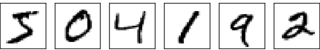
- Consider the \(784\) pixel values as the input values to a function.
- Is there a function \(y = f(x)\) whose output gives the digit number?
- Specifically, with \(x \in \R^{784}\) and \(y \in \R^{10}\) we want a function \(f(x)\) as follows:
\[ f(x) = \left\{ \begin{array}{cl} \bmat{1 & 0 & \cdots & 0} & \text{if } x \text{ is an image of a } 0 \\ \bmat{0 & 1 & \cdots & 0} & \text{if } x \text{ is an image of a } 1 \\ \vdots & \vdots \\ \bmat{0 & 0 & \cdots & 1} & \text{if } x \text{ is an image of a } 9 \end{array} \right. \]
- A neural network is a way to construct such a function \(f(x)\).
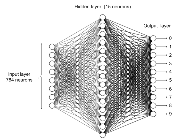
Network to identify handwritten digits
Pixel values: \(x \in \R^{784}\).
Outputs: \(a = f\left(x; {W}, {b}\right) \in \R^{10}\).
\({W}^{(2)} \in \R^{15 \times 784}\) \({b}^{(2)} \in \R^{15}\)
\({W}^{(3)} \in \R^{10 \times 15}\) \({b}^{(3)} \in \R^{10}\)
\(z^{(2)} = {W}^{(2)} x + {b}^{(2)}\) with output \(\sigma\left(z^{(2)}\right)\)
- \(x \in \R^{784}\)
- \({W}^{(2)} \in \R^{15 \times 784}\)
- \({b}^{(2)} \in \R^{15}\)
\(z^{(3)} = {W}^{(3)} \sigma\left(z^{(2)}\right) + {b}^{(3)}\) with output \(a = \sigma\left(z^{(3)}\right)\)
- \({W}^{(3)} \in \R^{10 \times 15}\)
- \({b}^{(3)} \in \R^{10}\)
Stochastic Gradient Descent
Let \(\mathcal{D} = \left(x^{(\ell)}, y^{(\ell)}\right)\) for \(\ell = 1, \ldots, n\) denote the image-label pairs in the MNIST data set.
We will use gradient descent to find \(W^{(2)} \in \R^{15 \times 784}\), \(b^{(2)} \in \R^{15}\), \(W^{(3)} \in \R^{10 \times 15}\), \(b^{(3)} \in \R^{10}\) that minimize a cost function, say MSE loss: \[ \begin{aligned} C(W, b) &= \frac{1}{n} \sum_{\ell = 1}^n \frac{1}{2}\lVert f\left(x^{(\ell)}; W^{(2)}, b^{(2)}, W^{(3)}, b^{(3)}\right) - y^{(\ell)} \rVert^2 \\ &= \frac{1}{n}\sum_{(x,y) \in \mathcal{D}} \underbrace{\frac{1}{2} \lVert f\left(x; W^{(2)}, b^{(2)}, W^{(3)}, b^{(3)}\right) - y \rVert^2}_{C_{x, y}} \end{aligned} \]
Computational Challenges
As \(C(W, b) = \frac{1}{n}\sum_{\ell = 1}^n C_{x^\ell, y^\ell}\), we need to compute \[ \nabla C(W, b) = \frac{1}{n}\sum_{\ell = 1}^n \nabla C_{x^{(\ell)}, y^{(\ell)}} \in \R^{11,935}. \]
In other words, for each update of the weights and biases, we need to compute \[ \nabla \left(\frac{1}{2} \lVert f\left(x; W^{(2)}, b^{(2)}, W^{(3)}, b^{(3)}\right) - y \rVert^2\right) \in \R^{11,935} \] for each training image!
Notice that \[ \frac{1}{n} \sum_{\ell = 1}^n \nabla \left( \frac{1}{2}\lVert f\left(x^{(\ell)}; W^{(2)}, b^{(2)}, W^{(3)}, b^{(3)}\right) - y^{(\ell)} \rVert^2 \right) \] is an average value of the gradient over all the training images.
As \(n \simeq 50,000\), perhaps we can get a good estimate of the average gradient using (say) \(100\) training images?
- Randomly shuffle the MNIST dataset \(\mathcal{D} = \left\{ \left(x^{(1)}, y^{(1)}\right), \ldots, \left(x^{(50,000)}, y^{(50,000)}\right) \right\}\)
- Let \(m = 100\) be the size of the mini-batch.
- Denote by \(B^{(k)} = \left\{ \left(x^{(km+1)}, y^{(km+1)}\right), \ldots, \left(x^{((k+1)m)}, y^{((k+1)m)}\right) \right\}\) the \(k^{\text{th}}\) mini-batch for \(k = 0, \ldots, 499\).
- Continue to obtain \(\nicefrac{n}{m} = 500\) mini-batches.
The idea is that \[ \begin{aligned} \nabla C(W, b) &= \frac{1}{n} \sum_{\ell = 1}^n \nabla \left( \frac{1}{2}\lVert f\left(x^{(\ell)}; W^{(2)}, b^{(2)}, W^{(3)}, b^{(3)}\right) - y^{(\ell)} \rVert^2 \right) \\ &\approx \frac{1}{m} \sum_{j = km+1}^{(k+1)m} \nabla \left( \frac{1}{2}\lVert f\left(x^{(j)}; W^{(2)}, b^{(2)}, W^{(3)}, b^{(3)}\right) - y^{(j)} \rVert^2 \right) \quad \text{(sum over mini-batch k)} \end{aligned} \]
- Estimate the gradient of \(C(W, b)\) by averaging the gradients over a mini-batch of data.
- Greatly speeds up learning (updating the weights)
New updates \[ \begin{aligned} w_{ij}^{(2)} &\leftarrow w_{ij}^{(2)} - \frac{\eta}{m} \sum_{(x, y) \in B^{(k)}} \pd{C_{x,y}}{w_{ij}^{(2)}}, \quad b_{j}^{(2)} &\leftarrow b_{j}^{(2)} - \frac{\eta}{m} \sum_{(x, y) \in B^{(k)}} \pd{C_{x,y}}{b_{j}^{(2)}} \\ w_{ij}^{(3)} &\leftarrow w_{ij}^{(3)} - \frac{\eta}{m} \sum_{(x, y) \in B^{(k)}} \pd{C_{x,y}}{w_{ij}^{(3)}}, \quad b_{j}^{(3)} &\leftarrow b_{j}^{(3)} - \frac{\eta}{m} \sum_{(x, y) \in B^{(k)}} \pd{C_{x,y}}{b_{j}^{(3)}} \end{aligned} \]
- After running through all the mini-batches, we have updated the weights \(\nicefrac{n}{m} = 500\) times and gone through all the MNIST data once.
- This is called an epoch of training.
- Next epoch: Reshuffle the MNIST data and repeat the above.
- After many epochs of training, we hope the neural network can identify handwritten digits.
Network Structure
We have the following network structure

corresponding to the following equations \[ \begin{aligned} z^{(2)} &= W^{(2)} a^{(1)} + b^{(2)}, \quad a^{(2)} = \sigma(z^{(2)}) \\ z^{(3)} &= W^{(3)} a^{(2)} + b^{(3)}, \quad a^{(3)} = \sigma(z^{(3)}) \end{aligned} \]
Let the cost function be \[ C(W, b) = \frac{1}{2} \lVert a^{(3)} - y \rVert^2 = \frac{1}{2} \sum_{j=1}^{n_o} (a_j^{(3)} - y_j)^2. \]
Back-propagation algorithm: Systematic way to compute \[ \begin{aligned} &\pd{C}{w_{ij}^{(3)}}, \quad \pd{C}{b_{j}^{(3)}}, \quad \text{for } i = 1, 2, \ldots, n_o, \; j = 1, 2, \ldots, n_h \\ &\pd{C}{w_{ij}^{(2)}}, \quad \pd{C}{b_{j}^{(2)}}, \quad \text{for } i = 1, 2, \ldots, n_h, \; j = 1, 2, \ldots, n_I. \end{aligned} \]
Key trick: First compute \[ \delta^{(3)} = \pd{C}{z^{(3)}} = \bmat{ \pd{C}{z_1^{(3)}} \\ \pd{C}{z_2^{(3)}} \\ \vdots \\ \pd{C}{z_{n_o}^{(3)}} }, \quad \delta^{(2)} = \pd{C}{z^{(2)}} = \bmat{ \pd{C}{z_1^{(2)}} \\ \pd{C}{z_2^{(2)}} \\ \vdots \\ \pd{C}{z_{n_h}^{(2)}} }. \]
Compute \(\delta^{(3)} \triangleq \pd{C}{z^{(3)}}\)
Let’s start chasing the signal. Note first that
\[ \pd{C}{a_j^{(3)}} = \pd{}{a_j^{(3)}} \left( \frac{1}{2} \sum_{k=1}^{n_o} (a_k^{(3)} - y_k)^2 \right) = (a_j^{(3)} - y_j). \]
so that
\[ \pd{C}{z_j^{(3)}} = \pd{C}{a_j^{(3)}} \pd{a_j^{(3)}}{z_j^{(3)}} = \pd{C}{a_j^{(3)}} \sigma'(z_j^{(3)}) = \left(a_j^{(3)} - y_j\right) \sigma'(z_j^{(3)}). \]
In matrix form
\[ \delta^{(3)} = \underbrace{\left(a^{(3)} - y\right)}_{\nabla_a C = \pd{C}{a^{(3)}}} \odot \sigma'(z^{(3)}) \tag{1}\]
Compute \(\delta^{(2)} \triangleq \pd{C}{z^{(2)}}\)
By the chain rule, we have
\[ \bmat{ \pd{C}{a_1^{(2)}} & \pd{C}{a_2^{(2)}} & \cdots & \pd{C}{a_{n_h}^{(2)}} } = \underbrace{\bmat{ \pd{C}{z_1^{(3)}} & \pd{C}{z_2^{(3)}} & \cdots & \pd{C}{z_{n_o}^{(3)}} }}_{\left(\delta^{(3)}\right)^\top} \underbrace{\bmat{ \pd{z_1^{(3)}}{a_1^{(2)}} & \pd{z_2^{(3)}}{a_1^{(2)}} & \cdots & \pd{z_{n_o}^{(3)}}{a_1^{(2)}} \\ \pd{z_1^{(3)}}{a_2^{(2)}} & \pd{z_2^{(3)}}{a_2^{(2)}} & \cdots & \pd{z_{n_o}^{(3)}}{a_2^{(2)}} \\ \vdots & \vdots & \ddots & \vdots \\ \pd{z_1^{(3)}}{a_{n_h}^{(2)}} & \pd{z_2^{(3)}}{a_{n_h}^{(2)}} & \cdots & \pd{z_{n_o}^{(3)}}{a_{n_h}^{(2)}} }}_{W^{(3)}} \]
Another application of the chain rule gives
\[ \begin{aligned} \underbrace{\bmat{ \pd{C}{z_1^{(2)}} & \pd{C}{z_2^{(2)}} & \cdots & \pd{C}{z_{n_h}^{(2)}} }}_{\left(\delta^{(2)}\right)^\top} &= \bmat{ \pd{C}{a_1^{(2)}}\pd{a_1^{(2)}}{z_1^{(2)}} & \pd{C}{a_2^{(2)}}\pd{a_2^{(2)}}{z_2^{(2)}} & \cdots & \pd{C}{a_{n_h}^{(2)}}\pd{a_{n_h}^{(2)}}{z_{n_h}^{(2)}} } \\ &= \bmat{ \pd{C}{a_1^{(2)}}\sigma'(z_1^{(2)}) & \pd{C}{a_2^{(2)}}\sigma'(z_2^{(2)}) & \cdots & \pd{C}{a_{n_h}^{(2)}}\sigma'(z_{n_h}^{(2)}) } \\ &= \underbrace{\bmat{ \pd{C}{a_1^{(2)}} & \pd{C}{a_2^{(2)}} & \cdots & \pd{C}{a_{n_h}^{(2)}} }}_{\left(\delta^{(3)}\right)^\top W^{(3)}} \odot \bmat{ \sigma'(z_1^{(2)}) & \sigma'(z_2^{(2)}) & \cdots & \sigma'(z_{n_h}^{(2)}) } \end{aligned} \]
Taking the transpose, we obtain \[ \delta^{(2)} = \left(W^{(3)}\right)^\top \delta^{(3)} \odot \sigma'(z^{(2)}). \tag{2}\]
Compute \(\pd{C}{b_{j}^{(3)}}\)
\[ \begin{aligned} \pd{C}{b_j^{(3)}} = \sum_{k=1}^{n_o} \pd{C}{z_k^{(3)}} \pd{z_k^{(3)}}{b_j^{(3)}} &= \pd{C}{z_j^{(3)}}\pd{z_j^{(3)}}{b_j^{(3)}} \quad \text{as } z_k^{(3)} = \sum_{\ell=1}^{n_h} w_{k\ell}^{(3)} a_{\ell}^{(2)} + b_k^{(3)} \\ &= \pd{C}{z_j^{(3)}} \cdot 1 \quad \text{as } z_j^{(3)} = \sum_{\ell=1}^{n_h} w_{j\ell}^{(3)} a_{\ell}^{(2)} + b_j^{(3)}. \end{aligned} \]
More succinctly,
\[ \pd{C}{b^{(3)}} = \bmat{ \pd{C}{b_1^{(3)}} \\ \pd{C}{b_2^{(3)}} \\ \vdots \\ \pd{C}{b_{n_o}^{(3)}} } = \bmat{ \pd{C}{z_1^{(3)}} \\ \pd{C}{z_2^{(3)}} \\ \vdots \\ \pd{C}{z_{n_o}^{(3)}} } = \delta^{(3)}. \tag{3}\]
Compute \(\pd{C}{w_{ij}^{(3)}}\)
\[ \begin{alignedat}{2} \pd{C}{w_{ij}^{(3)}} &= \mathrlap{\sum_{k=1}^{n_o} \pd{C}{z_k^{(3)}} \pd{z_k^{(3)}}{w_{ij}^{(3)}}} \\ &= \pd{C}{z_j^{(3)}} \pd{z_j^{(3)}}{w_{ij}^{(3)}} && \quad \text{as} \quad z_k^{(3)} = \sum_{\ell=1}^{n_h} w_{k\ell}^{(3)} a_{\ell}^{(2)} + b_k^{(3)} \\ &= \pd{C}{z_j^{(3)}} \cdot a_i^{(2)} && \quad \text{as} \quad z_j^{(3)} = \sum_{\ell=1}^{n_h} w_{j\ell}^{(3)} a_{\ell}^{(2)} + b_j^{(3)}. \end{alignedat} \]
More succinctly,
\[ \pd{C}{W^{(3)}} = \bmat{ \pd{C}{w_{11}^{(3)}} & \pd{C}{w_{12}^{(3)}} & \cdots & \pd{C}{w_{1n_h}^{(3)}} \\ \pd{C}{w_{21}^{(3)}} & \pd{C}{w_{22}^{(3)}} & \cdots & \pd{C}{w_{2n_h}^{(3)}} \\ \vdots & \vdots & \ddots & \vdots \\ \pd{C}{w_{n_o1}^{(3)}} & \pd{C}{w_{n_o2}^{(3)}} & \cdots & \pd{C}{w_{n_on_h}^{(3)}} } = \bmat{ \pd{C}{z_1^{(3)}} \\ \pd{C}{z_2^{(3)}} \\ \vdots \\ \pd{C}{z_{n_o}^{(3)}} } \bmat{ a_1^{(2)} & a_2^{(2)} & \cdots & a_{n_h}^{(2)} } = \delta^{(3)} \left(a^{(2)}\right)^\top. \tag{4}\]
Compute \(\pd{C}{b_{j}^{(2)}}\)
\[ \begin{aligned} \pd{C}{b_j^{(2)}} = \sum_{k=1}^{n_h} \pd{C}{z_k^{(2)}} \pd{z_k^{(2)}}{b_j^{(2)}} &= \pd{C}{z_j^{(2)}}\pd{z_j^{(2)}}{b_j^{(2)}} \quad \text{as } z_k^{(2)} = \sum_{\ell=1}^{n_I} w_{k\ell}^{(2)} a_{\ell}^{(1)} + b_k^{(2)} \\ &= \pd{C}{z_j^{(2)}} \cdot 1 \quad \text{as } z_j^{(2)} = \sum_{\ell=1}^{n_I} w_{j\ell}^{(2)} a_{\ell}^{(1)} + b_j^{(2)}. \end{aligned} \]
More succinctly,
\[ \pd{C}{b^{(2)}} = \bmat{ \pd{C}{b_1^{(2)}} \\ \pd{C}{b_2^{(2)}} \\ \vdots \\ \pd{C}{b_{n_h}^{(2)}} } = \bmat{ \pd{C}{z_1^{(2)}} \\ \pd{C}{z_2^{(2)}} \\ \vdots \\ \pd{C}{z_{n_h}^{(2)}} } = \delta^{(2)}. \tag{5}\]
Compute \(\pd{C}{w_{ij}^{(2)}}\)
\[ \begin{alignedat}{2} \pd{C}{w_{ij}^{(2)}} &= \mathrlap{\sum_{k=1}^{n_h} \pd{C}{z_k^{(2)}} \pd{z_k^{(2)}}{w_{ij}^{(2)}}} \\ &= \pd{C}{z_j^{(2)}} \pd{z_j^{(2)}}{w_{ij}^{(2)}} && \quad \text{as} \quad z_k^{(2)} = \sum_{\ell=1}^{n_I} w_{k\ell}^{(2)} a_{\ell}^{(1)} + b_k^{(2)} \\ &= \pd{C}{z_j^{(2)}} \cdot a_i^{(1)} && \quad \text{as} \quad z_j^{(2)} = \sum_{\ell=1}^{n_I} w_{j\ell}^{(2)} a_{\ell}^{(1)} + b_j^{(2)}. \end{alignedat} \]
More succinctly,
\[ \pd{C}{W^{(2)}} = \bmat{ \pd{C}{w_{11}^{(2)}} & \pd{C}{w_{12}^{(2)}} & \cdots & \pd{C}{w_{1n_I}^{(2)}} \\ \pd{C}{w_{21}^{(2)}} & \pd{C}{w_{22}^{(2)}} & \cdots & \pd{C}{w_{2n_I}^{(2)}} \\ \vdots & \vdots & \ddots & \vdots \\ \pd{C}{w_{n_h1}^{(2)}} & \pd{C}{w_{n_h2}^{(2)}} & \cdots & \pd{C}{w_{n_hn_I}^{(2)}} } = \bmat{ \pd{C}{z_1^{(2)}} \\ \pd{C}{z_2^{(2)}} \\ \vdots \\ \pd{C}{z_{n_h}^{(2)}} } \bmat{ a_1^{(1)} & a_2^{(1)} & \cdots & a_{n_I}^{(1)} } = \delta^{(2)} \left(a^{(1)}\right)^\top. \tag{6}\]
Equations of Back Propagation
\[ C = \frac{1}{2} \| a^{(3)} - y \|^2 = \frac{1}{2} \sum_{j=1}^{n_o} (a_j^{(3)} - y_j)^2 \]
By Equation 1 \[ \delta^{(3)} = \nabla_a C \odot \sigma'(z^{(3)}) = (a^{(3)} - y) \odot \sigma'(z^{(3)}) \]
By Equation 3 \[ \pd{C}{b^{(3)}} = \delta^{(3)} \]
By Equation 4 \[ \pd{C}{W^{(3)}} = \delta^{(3)} (a^{(2)})^\top \]
By Equation 2 \[ \delta^{(2)} = (W^{(3)})^\top \delta^{(3)} \odot \sigma'(z^{(2)}) \]
By Equation 5 \[ \pd{C}{b^{(2)}} = \delta^{(2)} \]
By Equation 6 \[ \pd{C}{W^{(2)}} = \delta^{(2)} (a^{(1)})^\top \]