Week 2: Introduction to Learning
Image credits: Understanding Deep Learning by Simon J. D. Prince, [CC BY 4.0]
Image credits: Understanding Deep Learning by Simon J. D. Prince, [CC BY 4.0]

Supervised Learning
- Define a mapping from input to output
- Learn this mapping from paired input/output data examples
Regression

Graph Regression

Text Classification

Music Genre Classification

Image Classification

What is a supervised learning model?

- An equation relating input (age) to output (height)
- Search through a family of possible equations to find one that fits training data well
- Deep neural networks are just a very flexible family of equations
- Fitting deep neural networks = “Deep Learning”
Image Segmentation

- Multivariate binary classification problem (many outputs, two discrete classes)
- Convolutional encoder-decoder network
Depth Estimation

- Multivariate regression problem (many output, continuous)
- Convolutional encoder-decoder network
Pose Estimation

- Multivariate regression problem (many output, continuous)
- Convolutional encoder-decoder network
- Regression: continuous numbers as output
- Classification: discrete classes as output
- Two class and multiclass classification are treated somewhat differently.
- Univariate: one output
- Multivariate: more than one output
Translation
![]()
Image Captioning
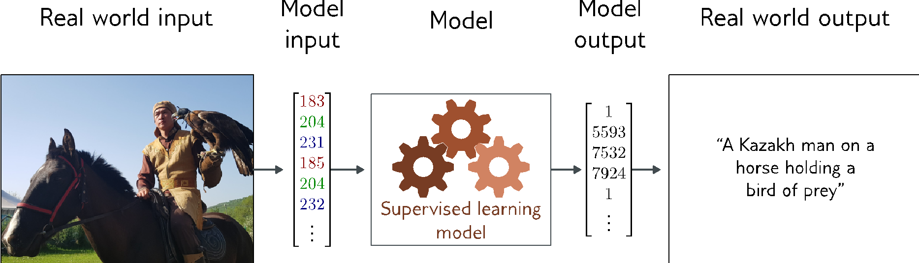
Image Generation from Text

All these examples have in common:
- Very complex relationship between input and ouput
- Sometimes there may be many possible valid answers
- However, outputs (and sometimes inputs) obey certain rules (e.g. grammar)
The idea might be
- Learn the “grammar” of the data from unlabeled examples
- Here we can use a gargantuan amount of data (unlabeled)
- This makes the supervised learning task easier by having a lot of knowledge of possible outputs
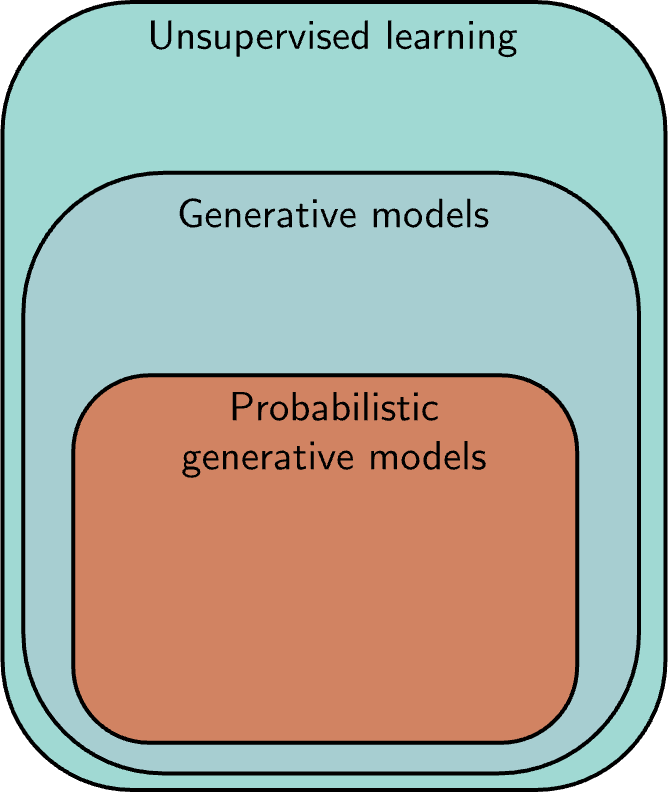
Unsupervised Learning
- Learning about a dataset without labels: e.g. clustering
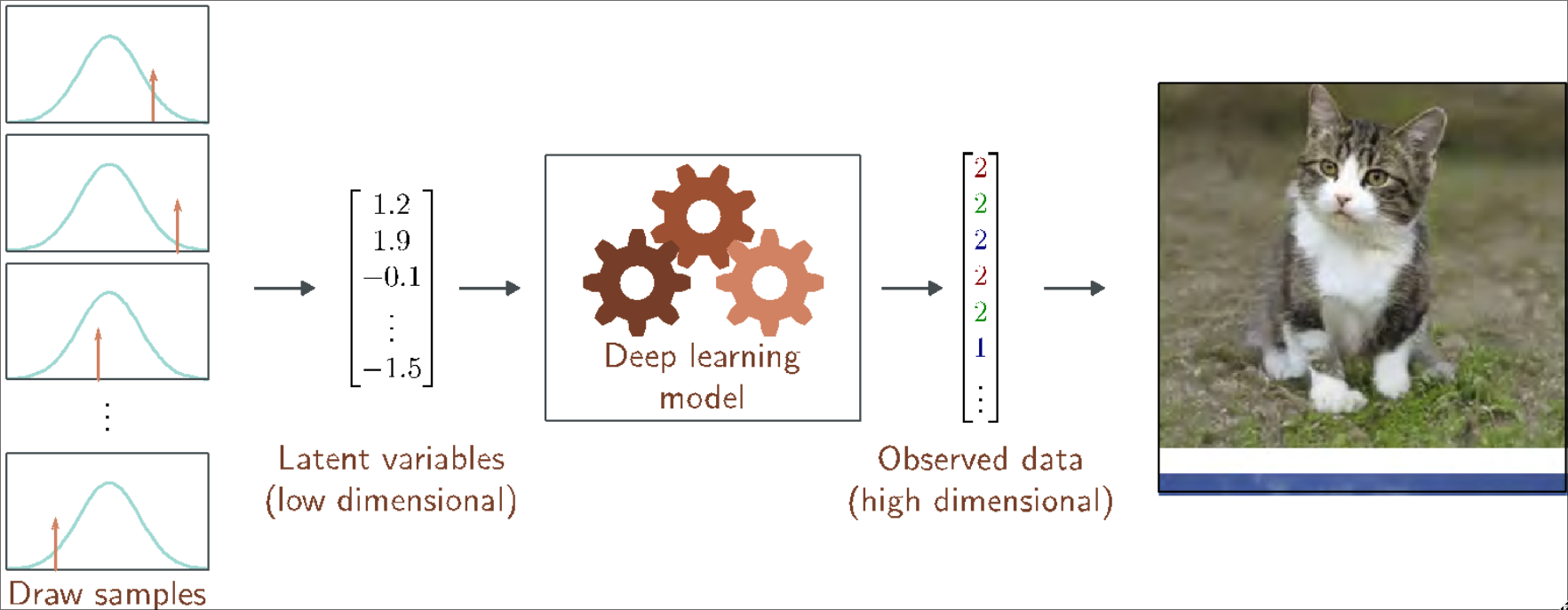
- Generative models can create examples: e.g. diffusion models
- PGMs learn distribution over data: e.g. VAEs, normalizing flows
Latent Variables
Reinforcement Learning

States are valid positions of the chess board
Actions at a given position are valid possible moves
Positive rewards for taking pieces, negative rewards for losing them
Goal: take actions to change the state so that you receive rewards
You don’t receive any data - you have to explore the environment yourself to gather data as you go.
Why is this difficult?
- Stochastic
- Make the same move twice, the opponent might not do the same thing
- Rewards also stochastic (opponent does or does not take your piece)
- Temporal credit assignment problem
- Did we get the reward b/c of this move or b/c/ we made good tactical decisions somewhere in the past?
- Exploration-exploitation trade-off
- If we found a good opening, should we stick to it?
- Should we try other things, hoping for something better?
- Supervised learning model defined a mapping from one or more inputs to one or more outputs
- The model is a family of mathematical equations
- Computing the outputs given the inputs is termed inference
- Input: age and milage of a second-hand Toyota Prius
- Output: estimated price of car
- Model also includes parameters
- Parameters affect the outcome of the model (equation)
- Training a model: finding parameters that predict the outputs “well”
- Given inputs for a training dataset of input/output pairs
Notation
- Input: \(\bm{x} \in \R^n\)
- Output: \(\bm{y} \in \R^m\)
- Model: \(\bm{y} = \bm{f}(\bm{x}; \bm{\phi})\)
- Parameters: \(\bm{\phi} \in \R^p\)
Loss function
- Training dataset: \(I\) pairs of input/output examples: \(\left\{ \bm{x}_i, \bm{y}_i \right\}_{i=1}^I\)
- Loss function or cost function measures how bad the model is: \[ \mc{L}\left(\bm{\phi}, \underbrace{\bm{f}(\bm{x}; \bm{\phi})}_{\text{model}}, \left\{ \bm{x}_i, \bm{y}_i \right\}_{i=1}^I\right) \]
or for short \(\mc{L}(\bm{\phi})\)
Training
- Find the parameters that minimize the loss: \[ \hat{\bm{\phi}} = \argmin_{\bm{\phi}}\; \mc{L}(\bm{\phi}) \]
Testing
- To test the model, run on a separate test dataset of input/output pairs
- See how well it generalizes to new data
Regression
- Univariate regression problem (one output, real value)
- Fully connected network
Example

- Loss function \[ \mathcal{L}(\bm{\phi}) = \sum_{i=1}^I \left( f(x_i; \bm{\phi}) - y_i \right)^2 = \sum_{i=1}^I \left(\phi_0 + \phi_1x_i - y_i \right)^2 \]

- Training performed by gradient descent
- 1D regression model is obviously limited
- Want to be able to describe input/output that are not lines
- Want multiple inputs
- Want multiple outputs
- Shallow neural nets
- Flexible enough to describe arbitrarily complex input/output mappings
- Can have as many inputs and outputs as we want
Example shallow neural net
\[ y = f(x; \bm{\phi}) = \phi_0 + \phi_1 \sigma(\theta_{10} + \theta_{11}x) + \phi_2\sigma(\theta_{20} + \theta_{21}x) + \phi_3\sigma(\theta_{30} + \theta_{31}x), \tag{1}\]
where \(\sigma: \R \to \R\) is the rectified linear unit, which is a particular kind of activation function
\[ \sigma(z) = \operatorname{ReLU}(z) = \begin{cases} 0, & z < 0 \\ z, & z \geq 0 \end{cases} \]

This model has \(10\) parameters: \(\bm{\phi} = \{\phi_0, \phi_1, \phi_2, \phi_3, \theta_{10}, \theta_{11}, \theta_{20}, \theta_{21}, \theta_{30}, \theta_{31}\}\).
- Represents a family of functions
- Parameters determine particular function
- Given parameters, can perform inference (run equation)
- Given training set \(\{\bm{x}_i, \bm{y}_i\}_{i=1}^I\), define loss function \(\mc{L}\)
- Change parameters to minimize loss function


Depicting neural nets

Universal approximation theorem
Generalizing from three hidden units to \(D\) hidden units, we have the \(d^{\text{th}}\) hidden unit is described by
\[ h_d = \sigma(\theta_{d0} + \theta_{d1}x), \]
and these are combined linearly (more precisely affinely) to create the output:
\[ y = \phi_0 + \sum_{d=1}^D \phi_dh_d. \]
With enough network capacity (number of hidden units), a shallow network can describe any continuous function on a compact subset of \(\R^D\) to arbitrary precision.

Two inputs
- 2 inputs, 3 hidden units, 1 output
\[ \begin{split} h_1 &= \sigma(\theta_{10} + \theta_{11}x_1 + \theta_{12}x_2) \\ h_2 &= \sigma(\theta_{20} + \theta_{21}x_1 + \theta_{22}x_2) \\ h_3 &= \sigma(\theta_{30} + \theta_{31}x_1 + \theta_{32}x_2) \end{split} \]
\[ y = \phi_0 + \phi_1h_1 + \phi_2h_2 + \phi_3h_3 \]

- What if there were two outputs, what would the would the contour lines of the second output look like as compared to j) above?
General case
- \(D_o\) outputs, \(D\) hidden units, \(D_i\) inputs
\[ h_d = \sigma\left(\theta_{d0} + \sum_{i=1}^{D_i}\theta_{di}x_i\right) \]
\[ y_j = \phi_{j0} + \sum_{d=1}^D\phi_{jd}h_d \]

Number of output regions
- In general, each output consists of \(D\) dimensional convex polytopes
- With two inputs, and three outputs, we saw there were seven polygons.

Number of regions created by \(D > D_i\) polytopes in \(D_i\) dimensions is \[ \sum_{j=0}^{D_i} \binom{D}{j}. \] Note that \[ 2^{D_i} < \sum_{j=0}^{D_i} \binom{D}{j} < 2^D. \]

Terminology

- y-offsets: biases
- slopes: weights
- every node connected every other: fully connected network
- no loops: feedforward network
- values after the activation functions: activations
- values before the activation functions: preactivations
- one hidden layer: shallow neural network
- more than one hidden layer: deep neural network
- number of hidden units \(\approx\) capacity
Other activation functions
