Diffusion and Flow Models
Credits: Introduction to Flow Matching and Diffusion Models by Peter Holderrieth
Credits: Introduction to Flow Matching and Diffusion Models by Peter Holderrieth
Flow Matching by Mario Gemoll
Credits: Introduction to Flow Matching and Diffusion Models by Peter Holderrieth
Flow Matching by Mario Gemoll
Credits: Introduction to Flow Matching and Diffusion Models by Peter Holderrieth
Flow Matching by Mario Gemoll
Credits: Introduction to Flow Matching and Diffusion Models by Peter Holderrieth
Credits: Introduction to Flow Matching and Diffusion Models by Peter Holderrieth
A new generation of AI systems are “creative” they generate new objects.
Goal of these notes:
- Flow and diffusion models from first principles.
- The minimal but necessary amount of mathematics for 1.
- How to implement and apply these algorithms.
From Generation to Sampling
Images
- Height \(H\) and Width \(W\)
- 3 color channels (RGB)
\[\mathbf{z} \in \mathbb{R}^{H \times W \times 3}\]
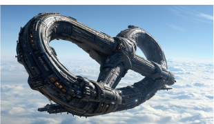
Videos
- \(T\) time frames
- Each frame is an image
\[\mathbf{z} \in \mathbb{R}^{T \times H \times W \times 3}\]

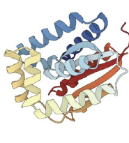
Molecular structures
- \(N\) atoms
- Each atom has 3 coordinates
\[\mathbf{z} \in \mathbb{R}^{N \times 3}\]
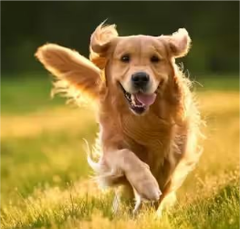
What does it mean to successfully generate something?
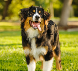
Prompt: “A picture of a dog”
 Useless
(Impossible)
 Bad
Bad
(Rare)
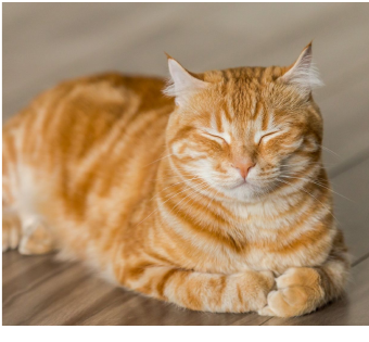 Wrong animal
(Unlikely)
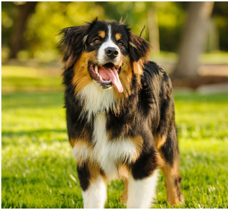 Great!
(Very likely)
Generation as Sampling the Data Distribution
We think of the objects we want to generate as following a data distribution \(p_{\text{data}}\). This is a probability density function:
\[p_{\text{data}} : \mathbb{R}^d \to \mathbb{R}_{\ge 0}, \quad \mathbf{z} \mapsto p_{\text{data}}(\mathbf{z})\]
Crucial Note: In practice, we do not know the analytical form of \(p_{\text{data}}\)!
In this framework, generation means sampling from the data distribution:
\(\mathbf{z} \sim p_{\text{data}}\) \(\quad \implies \quad\) \(\mathbf{z} =\)
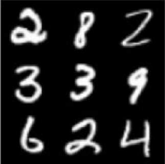
What consists a Dataset?
Since we don’t know \(p_{\text{data}}\), we rely on a dataset: a finite collection of samples drawn from it.
- Images: Publicly available images from the internet (e.g., LAION, ImageNet).
- Videos: Large-scale video repositories (e.g., YouTube).
- Molecular structures: Scientific repositories (e.g., Protein Data Bank).
Mathematically, a dataset is a collection: \[\{\mathbf{z}_1, \dots, \mathbf{z}_N\} \sim p_{\text{data}}\]
Conditional Generation
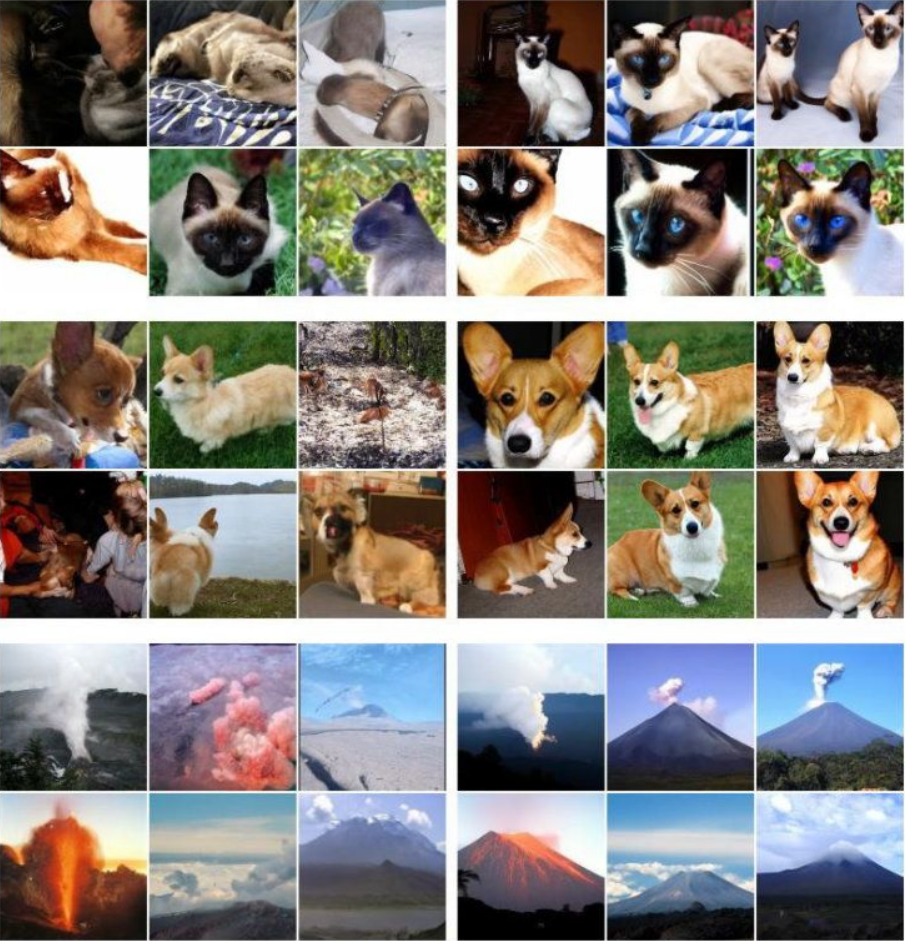
Standard (unconditional) generation samples from \(p_{\text{data}}\). However, we often want to condition our generation on a prompt or label \(y\) (e.g., \(y = \text{"Dog"}\)).
Unconditional (\(p_{\text{data}}\))
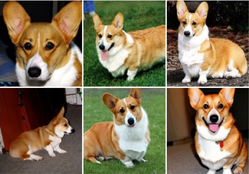
Fixed prompt “Dog” — diverse samples of the same category:
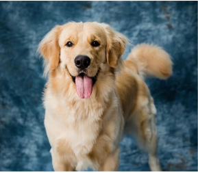
Conditional (\(p_{\text{data}}(\cdot|y)\))
Changing \(y\) gives different targeted categories:

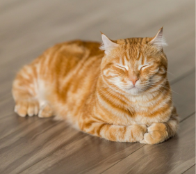
Conditional generation means sampling the conditional data distribution: \[ \color{#a71d5d}{\mathbf{z} \sim p_{\text{data}}(\cdot | y)} \]
We will first focus on unconditional generation and then learn how to translate an unconditional model to a conditional one.
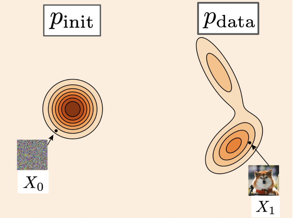
Generative Models as Transformers
A generative model converts samples from a simple initial distribution \(p_{\text{init}}\) into samples from the complex data distribution \(p_{\text{data}}\).
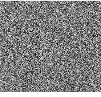
Initial State
\[\mathbf{x} \sim p_{\text{init}}\]
\(\mathcal{N}(0, \mathbf{I}_d)\)

\(\implies\)
Generative Model
\(\implies\)
Target Sample
\[\mathbf{z} \sim p_{\text{data}}\]
(Real Object)

Existence and Uniqueness Theorem ODEs
Theorem (Picard–Lindelöf theorem): If the vector field \(u_t(x)\) is continuously differentiable with bounded derivatives, then a unique solution to the ODE
\[ X_0 = x_0, \quad \frac{\mathrm{d}}{\mathrm{d}t}X_t = u_t(X_t) \]
exists. In other words, a flow map exists. More generally, this is true if the vector field is Lipschitz.
Key takeaway: In the cases of practical interest for machine learning, unique solutions to ODE/flows exist.
Example: Linear ODE
Simple vector field:
\[ u_t(x) = -\theta x \quad (\theta > 0) \]
Claim: Flow is given by
\[ \psi_t(x_0) = \exp(-\theta t) x_0 \]
Proof:
Initial condition: \[ \psi_t(x_0) = \exp(0)x_0 = x_0 \]
ODE: \[ \frac{\mathrm{d}}{\mathrm{d}t} \psi_t(x_0) = \frac{\mathrm{d}}{\mathrm{d}t} \left(\exp(-\theta t) x_0\right) = -\theta \exp(-\theta t) x_0 = -\theta \psi_t(x_0) = u_t(\psi_t(x_0)) \]
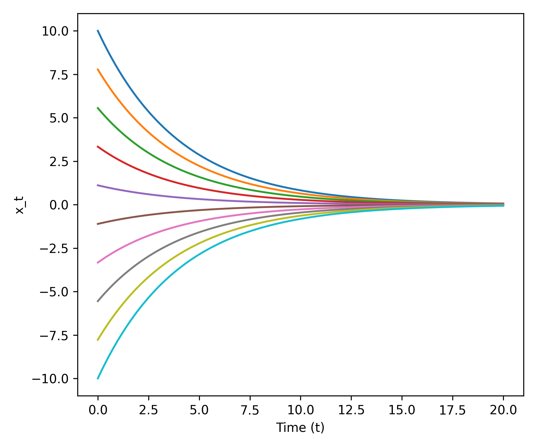
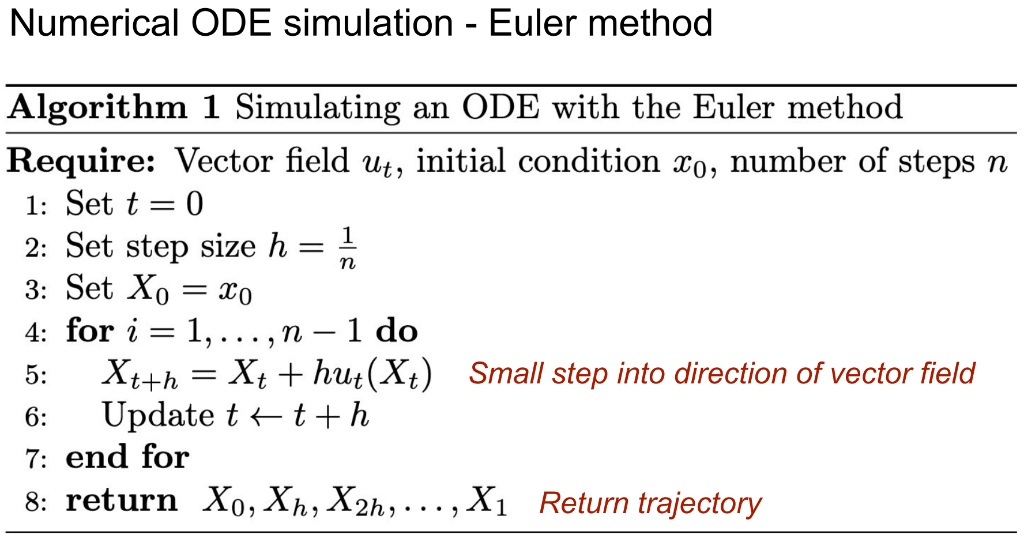
Euler Method: Coarse vs Fine Steps
Toy example
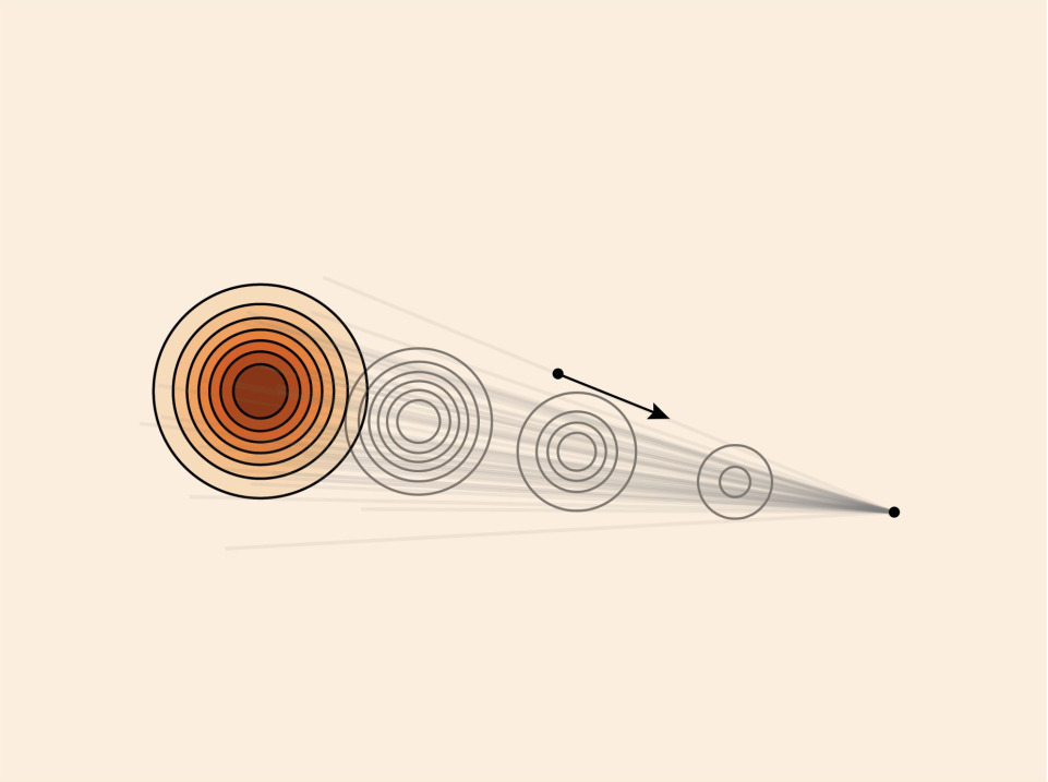
Brownian Motion or the Wiener Process
Brownian motion describes the random motion of particles in fluids or gases. It is basically a random walk. Mathematically it can be modeled as a Wiener process. For our purposes, we can think of this as a path starting at the origin at \(t = 0\), and then proceeding with step size \(h\), adding noise from a standard Gaussian scaled by \(\sqrt{h}\) at each step, until \(t = 1\):
\[ W_{t+h} = W_t + \sqrt{h}\epsilon_t, \quad \epsilon_t \sim \mathcal{N}(0, Id) \quad (t = 0, h, 2h, \dots, 1 - h) \]
Note: A single stochastic process can give rise to many trajectories as the evolution becomes random.
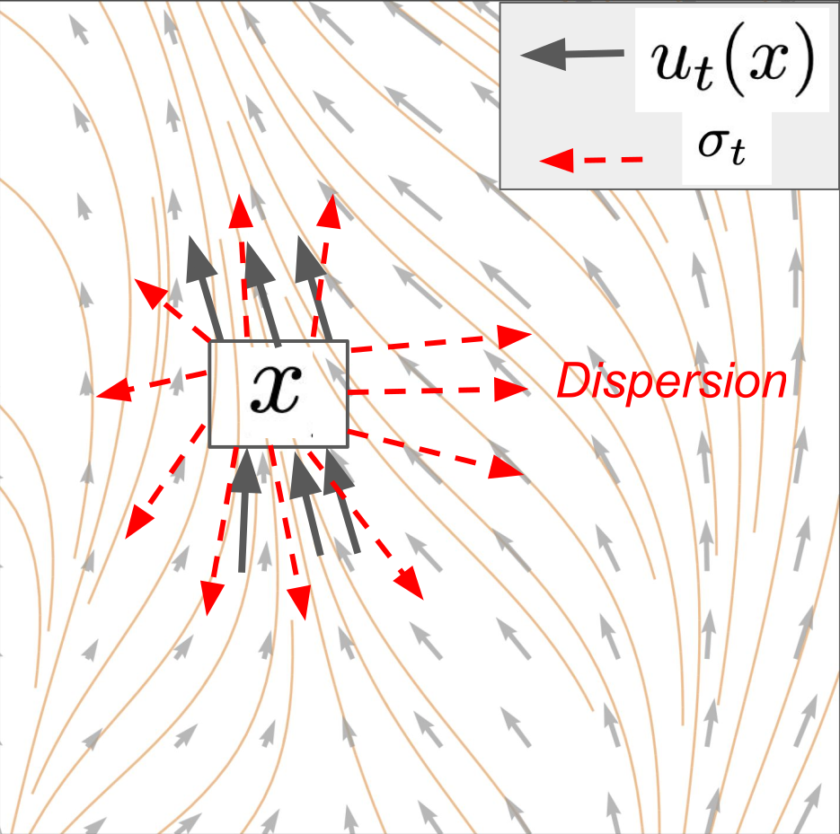
Stochastic Differential Equations (SDEs)
We can add some Brownian motion to the paths taken by particles moving along a vector field described by an ODE, which gives rise to the concept of a stochastic differential equation (SDE):
\[ \begin{align*} \mathrm{d}X_t &= u_t(X_t)\mathrm{d}t + \sigma_t \mathrm{d}W_t \\ X_0 &= x_0 \end{align*} \]
For the details about the \(\mathrm{d}X\) notation, see Holderrieth & Erives, 2025.
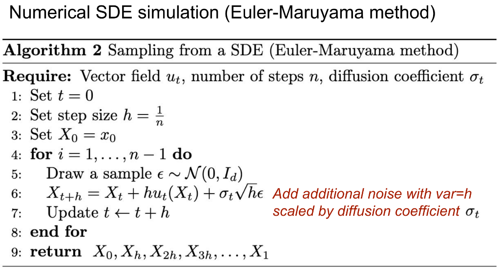
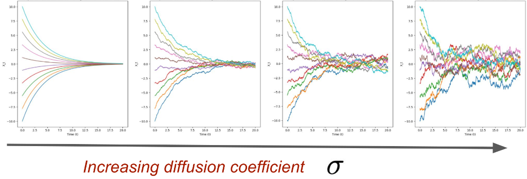
The \(\sigma_t\) in the above equation is called the diffusion coefficient and controls the amount of randomness (the ODE term \(u_t(X_t)\) is also called the drift coefficient).
Such an SDE can be approximated by the Euler-Maruyama method (basically the Euler method with some randomness added to it):
\[ x_{t+h} = x_t + h u_t(x_t) + \sqrt{h} \sigma_t \epsilon_t, \quad \epsilon_t \sim \mathcal{N}(0, I_d) \]
Existence and Uniqueness Theorem SDEs
Theorem: If the vector field \(u_t(x)\) is continuously differentiable with bounded derivatives and the diffusion coeff. is continuous, then a unique solution (in distribution) to the SDE
\[ X_0 = x_0, \quad \mathrm{d}X_t = u_t(X_t)\mathrm{d}t + \sigma_t\mathrm{d}W_t \]
exists. More generally, this is true if the vector field is Lipschitz.
Key takeaway: In the cases of practical interest for machine learning, unique solutions to SDEs exist.
Stochastic calculus class: Construct solutions via stochastic integrals and Ito-Riemann sums
Ornstein-Uhlenbeck Process
\[ \dd X_t = -\theta X_t \dd t + \sigma \dd W_t \]
Reminder: Flow and Diffusion Models
Flow
Model
Initialize:
\[X_0 \sim \underbrace{p_{\text{init}}}_{\color{#a30000}{\text{e.g. Gaussian}}}\]
ODE:
\[\mathrm{d}X_t = \underbrace{u_t^{\theta}(X_t)}_{\substack{\color{#a30000}{\text{neural network}} \\ \color{#a30000}{\text{vector field}}}}\mathrm{d}t\]
Diffusion
Model
Initialize:
\[X_0 \sim \underbrace{p_{\text{init}}}_{\color{#a30000}{\text{e.g. Gaussian}}}\]
SDE:
\[\mathrm{d}X_t = \underbrace{u_t^{\theta}(X_t)}_{\substack{\color{#a30000}{\text{neural network}} \\ \color{#a30000}{\text{vector field}}}}\mathrm{d}t + \underbrace{\sigma_t}_{\color{#a30000}{\text{diffusion coeff.}}}\mathrm{d}W_t\]
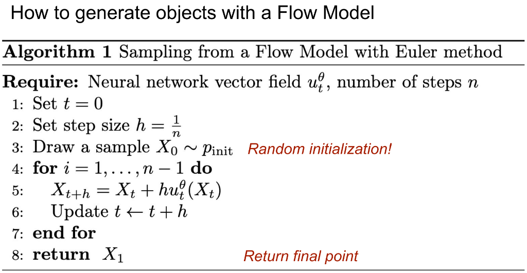
Next Step: Training a Flow Model
Training = Finding parameters \(\theta\) such that
\[\underbrace{X_0 \sim p_{\text{init}}}_{\color{#a30000}{\small\textit{Start with initial distribution}}}\]
\[\underbrace{\mathrm{d}X_t = u_t^{\theta}(X_t)\mathrm{d}t}_{\color{#a30000}{\small\textit{Follow along the vector field}}}\]
\(\Rightarrow\)
Implies
\[\underbrace{X_1 \sim p_{\text{data}}}_{\substack{\color{#a30000}{\small\textit{Distribution of final}} \\ \color{#a30000}{\small\textit{point = data dist.}}}}\]
The Flow Matching Matrix
Conditional
Probability Path
\(\rightarrow\)
Conditional
Vector Field
\(\rightarrow\)
Conditional
Flow Matching Loss
Marginal
Probability Path
\(\rightarrow\)
Marginal
Vector Field
\(\rightarrow\)
Marginal
Flow Matching Loss
“Conditional” = “Per single data point”
“Marginal” = “Across distribution of data points”
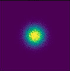
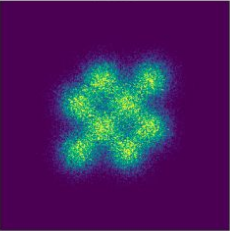
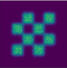
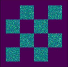
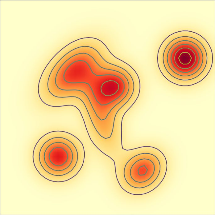
Probability Paths: The Path from Noise to Data
Noise
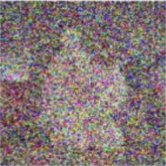
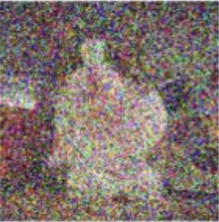
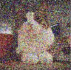

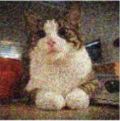

Data
\(t=0\)
\(\longleftarrow\) time \(\longrightarrow\)
\(t=1\)
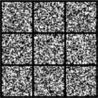
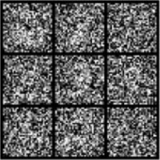
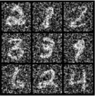
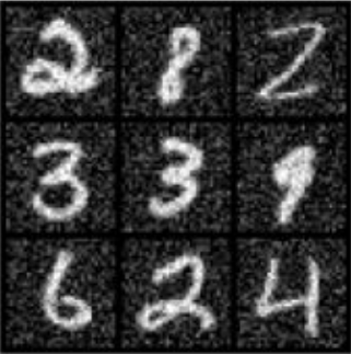
Conditional Probability Path \(p_t(\cdot | z)\)
\(p_{\text{init}}\)
\(t = 0.00\)
\(t = 0.25\)
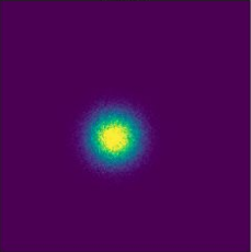
\(t = 0.50\)
\(t = 0.75\)
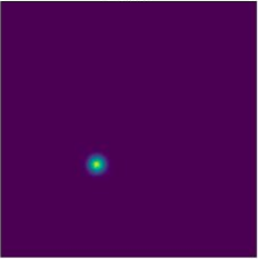
\(t = 1.00\)
\(z\)
↓
t=0
\(\longrightarrow\)
t=1
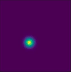
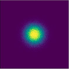
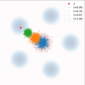
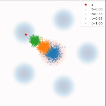
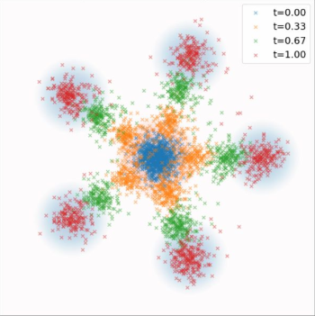
Conditional vs. Marginal Probability Path
Conditional Probability Path \(p_t(\cdot | z)\)
\(p_{\text{init}}\)
\(t=0.00\)
\(t=0.25\)
\(t=0.50\)
\(t=0.75\)
\(t=1.00\)
\(z\)
↓
\(p_{\text{init}}\)
\(t=0.00\)
\(t=0.25\)
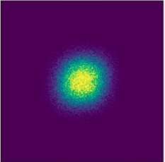
\(t=0.50\)
\(t=0.75\)
\(t=1.00\)
\(p_{\text{data}}\)
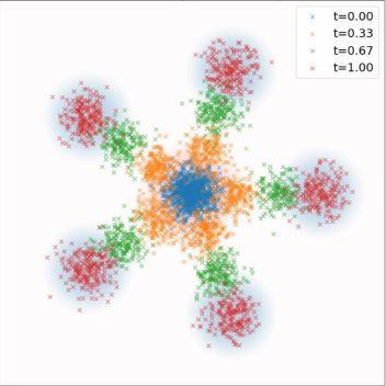
Marginal Probability Path \(p_t\)
Conditional Probability Path
| Notation | Key property | Gaussian example | |
|---|---|---|---|
| Conditional Probability Path | \(p_t(\cdot\|z)\) | Interpolates \(p_{\text{init}}\) and a data point \(z\) | \(\mathcal{N}(\alpha_t z,\, \beta_t^2 I_d)\) |
| Conditional Vector Field | \(u_t^c(x,z)\) |
Marginal Probability Path
| Notation | Key property | Formula | |
|---|---|---|---|
| Marginal Probability Path | \(p_t\) | Interpolates \(p_{\text{init}}\) and \(p_{\text{data}}\) | \(\int p_t(x\|z)\, p_{\text{data}}(z)\,\mathrm{d}z\) |
| Marginal Vector Field |
Example — Conditional Vector Field for Gaussian
\[u_t^{\text{target}}(x|z) = \left(\dot{\alpha}_t - \frac{\dot{\beta}_t}{\beta_t}\alpha_t\right)z + \frac{\dot{\beta}_t}{\beta_t}x\]
Proof Sketch:
Step 1: By checking ODE, show that the flow of the vector field is given by
\[\psi_t^{\text{target}}(x_0|z) = \alpha_t z + \beta_t x_0\]
Step 2: If \(X_0 = x_0 \sim \mathcal{N}(0, I_d)\) is random, then we know that then:
\[X_t = \psi_t(X_0|z) = \alpha_t z + \beta_t X_0 \sim \mathcal{N}(\alpha_t z,\, \beta_t^2 I_d) = p_t(\cdot|z)\]
Gaussian Conditional Probability Path And Conditional Vector Field
Figure credit: Yaron Lipman
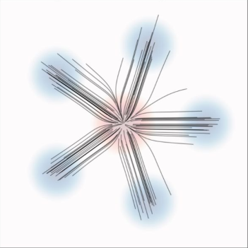
Ground truth
ODE samples
ODE Trajectories
\(p_t(\cdot|z)\)
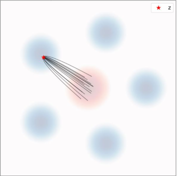
\(p_t\)
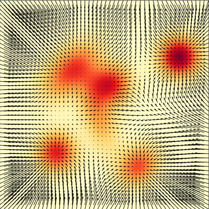
Continuity Equation
Randomly initialized ODE
Given: \(\quad X_0 \sim p_{\text{init}}, \qquad \dfrac{\mathrm{d}}{\mathrm{d}t}X_t = u_t(X_t)\)
Follow probability path:
\[X_t \sim p_t \qquad (0 \le t \le 1)\]
Marginals are \(p_t\)
\(\Longleftrightarrow\) equivalent
Continuity equation holds
\[\frac{\mathrm{d}}{\mathrm{d}t}p_t(x) = -\operatorname{div}(p_t u_t)(x)\]
PDE holds
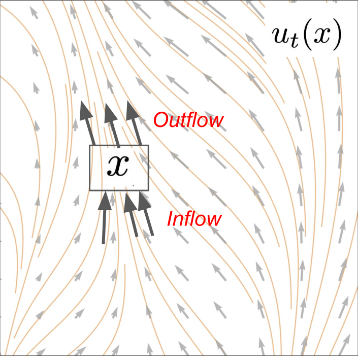
Continuity Equation
\[\frac{\mathrm{d}}{\mathrm{d}t}p_t(x) = -\operatorname{div}(p_t u_t)(x)\]
Change of probability mass at \(x\)
Outflow - inflow of probability mass from \(u\)
Conditional Flow Matching for Gaussian Probability Path
Prob. path
\(\mathcal{N}(\alpha_t z,\, \beta_t^2 I_d)\)
Conditional VF
\(u_t^{\text{target}}(x|z) = \left(\dot{\alpha}_t - \dfrac{\dot{\beta}_t}{\beta_t}\alpha_t\right)z + \dfrac{\dot{\beta}_t}{\beta_t}x\)
Noise Sampling
\(x \sim p_t(\cdot|z) \quad \Leftrightarrow \quad x = \alpha_t z + \beta_t \epsilon, \quad \epsilon \sim \mathcal{N}(0, I_d)\)
Plugging in Noise Sampling into CFM Loss results in:
\[ \begin{align} L_{\text{CFM}}(\theta) &= \mathbb{E}_{t \sim \text{Unif},\, z \sim p_{\text{data}},\, x \sim p_t(\cdot|z)} \left[\|u_t^\theta(x) - u_t^{\text{target}}(x|z)\|^2\right] \\ &= \mathbb{E}_{t \sim \text{Unif},\, z \sim p_{\text{data}},\, \epsilon \sim \mathcal{N}(0,I_d)} \left[\|u_t^\theta(\alpha_t z + \beta_t \epsilon) - u_t^{\text{target}}(\alpha_t z + \beta_t \epsilon|z)\|^2\right] \\ &= \mathbb{E}_{t \sim \text{Unif},\, z \sim p_{\text{data}},\, \epsilon \sim \mathcal{N}(0,I_d)} \left[\|\underbrace{u_t^\theta(\alpha_t z + \beta_t \epsilon)}_{\color{#a30000}{\textbf{noise+data}}} - \underbrace{(\dot{\alpha}_t z + \dot{\beta}_t \epsilon)}_{\color{#a30000}{\textbf{velocity}}}\|^2\right] \end{align} \]
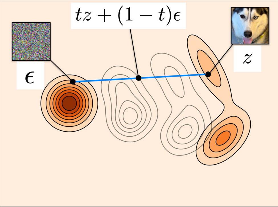
Straight Line Schedule
\[ \begin{align} L_{\text{CFM}}(\theta) &= \mathbb{E}_{t \sim \text{Unif},\, z \sim p_{\text{data}},\, \epsilon \sim \mathcal{N}(0,I_d)} \left[\|u_t^\theta(\alpha_t z + \beta_t \epsilon) - (\dot{\alpha}_t z + \dot{\beta}_t \epsilon)\|^2\right] \\ &= \mathbb{E}_{t \sim \text{Unif},\, z \sim p_{\text{data}},\, \epsilon \sim \mathcal{N}(0,I_d)} \left[\|\underbrace{u_t^\theta(tz + (1-t)\epsilon)}_{\substack{\color{#a30000}{\textbf{Linear interpolation}} \\ \color{#a30000}{\textbf{of noise and data}}}} - \underbrace{(z - \epsilon)}_{\substack{\color{#a30000}{\textbf{Difference between}} \\ \color{#a30000}{\textbf{noise and data}}}}\|^2\right] \end{align} \]
Example Flow Matching — Stable Diffusion 3

The neural network that generates these images was trained with the algorithm just shown
Reminder: Sampling Algorithm for Flow Model
The Flow Matching Matrix
Conditional
Probability Path
\(\rightarrow\)
Conditional
Vector Field
\(\rightarrow\)
Conditional
Flow Matching Loss
Marginal
Probability Path
\(\rightarrow\)
Marginal
Vector Field
\(\rightarrow\)
Marginal
Flow Matching Loss
Defines distributions from noise to data
Defines training target that we want to learn
Loss function that we want to minimize during training
Conditional Probability Path, Vector Field, and Flow Matching Loss
| Notation | Key property | Gaussian example | |
|---|---|---|---|
| Conditional Probability Path | \(p_t(\cdot\|z)\) | Interpolates \(p_{\text{init}}\) and a data point \(z\) | \(\mathcal{N}(\alpha_t z,\, \beta_t^1 I_d)\) |
| Conditional Vector Field | \(u_t^{\text{target}}(x\|z)\) | ODE follows conditional path | \(\left(\dot{\alpha}_t - \dfrac{\dot{\beta}_t}{\beta_t}\alpha_t\right)z + \dfrac{\dot{\beta}_t}{\beta_t}x\) |
| Conditional FM Loss | \(L_{\text{CFM}}(\theta)\) | Loss we minimize during training | \(\mathbb{E}_{t,z,x}\left[\|u_t^\theta(x) - u_t^{\text{target}}(x\|z)\|^1\right]\) |
All these objects are tractable. Just analytical formulas!
Marginal Probability Path, Vector Field, and Flow Matching Loss
| Notation | Key property | Formula | |
|---|---|---|---|
| Marginal Probability Path | \(p_t\) | Interpolates \(p_{\text{init}}\) and \(p_{\text{data}}\) | \(\int p_t(x\|z)\, p_{\text{data}}(z)\,\mathrm{d}z\) |
| Marginal Vector Field | \(u_t^{\text{target}}(x)\) | ODE follows marginal path | \(\int u_t^{\text{target}}(x\|z)\,\dfrac{p_t(x\|z)\,p_{\text{data}}(z)}{p_t(x)}\,\mathrm{d}z\) |
| Marginal FM Loss | \(L_{\text{FM}}(\theta)\) | Implicitly minimized via cond FM loss | \(\mathbb{E}_{t,z,x}\left[\|u_t^\theta(x) - u_t^{\text{target}}(x)\|^2\right]\) |
None of these objects are tractable. But we can still learn them!
Reminder: Conditional Probability Path and Conditional Vector Field
| Notation | Key property | Gaussian example | |
|---|---|---|---|
| Conditional Probability Path | \(p_t(\cdot\|z)\) | Interpolates \(p_{\text{init}}\) and a data point \(z\) | \(\mathcal{N}(\alpha_t z,\, \beta_t^2 I_d)\) |
| Conditional Vector Field | \(u_t^{\text{target}}(x\|z)\) | ODE follows conditional path | \(\left(\dot{\alpha}_t - \dfrac{\dot{\beta}_t}{\beta_t}\alpha_t\right)z + \dfrac{\dot{\beta}_t}{\beta_t}x\) |
Reminder: Marginal Probability Path and Marginal Vector Field
| Notation | Key property | Formula | |
|---|---|---|---|
| Marginal Probability Path | \(p_t\) | Interpolates \(p_{\text{init}}\) and \(p_{\text{data}}\) | \(\int p_t(x\|z)\, p_{\text{data}}(z)\,\mathrm{d}z\) |
| Marginal Vector Field | \(u_t^{\text{target}}(x)\) | ODE follows marginal path | \(\int u_t^{\text{target}}(x\|z)\,\dfrac{p_t(x\|z)\,p_{\text{data}}(z)}{p_t(x)}\,\mathrm{d}z\) |
Algorithm 3: Flow Matching Training Procedure (General)
Reminder: Sampling Algorithm for Flow Model
Score Functions = Gradients of the log-likelihood
Log-likelihood: \(\log q(x)\)
Score function: \(\nabla \log q(x)\)
Example — Score of Gaussian Probability Path
\[\nabla \log p_t(x|z) = -\frac{1}{\beta_t^2}x + \frac{\alpha_t}{\beta_t^2}z\]
Proof:
\[p_t(x|z) = \mathcal{N}(x;\, \alpha_t z, \beta_t^2 I_d) = \frac{1}{(2\pi)^{d/2}\beta_t^d} \exp\!\left(-\frac{1}{2\beta_t^2}\|x - \alpha_t z\|^2\right)\]
\[\log p_t(x|z) = \log \mathcal{N}(x;\, \alpha_t z, \beta_t^2 I_d) = -\frac{d}{2}\log(2\pi) - d\log\beta_t - \frac{1}{2\beta_t^2}\|x - \alpha_t z\|^2\]
\[\nabla \log p_t(x|z) = \nabla \log \mathcal{N}(x;\, \alpha_t z, \beta_t^2 I_d) = -\frac{x - \alpha_t z}{\beta_t^2}\]
Conditional Probability Path, Vector Field, and Score
| Notation | Key property | Gaussian example | |
|---|---|---|---|
| Conditional Probability Path | \(p_t(\cdot\|z)\) | Interpolates \(p_{\text{init}}\) and a data point \(z\) | \(\mathcal{N}(\alpha_t z,\, \beta_t^2 I_d)\) |
| Conditional Vector Field | \(u_t^{\text{target}}(x\|z)\) | ODE follows conditional path | \(\left(\dot{\alpha}_t - \dfrac{\dot{\beta}_t}{\beta_t}\alpha_t\right)z + \dfrac{\dot{\beta}_t}{\beta_t}x\) |
| Conditional Score Function | \(\nabla \log p_t(x\|z)\) | Gradient of log-likelihood | \(\dfrac{\alpha_t}{\beta_t^2}z - \dfrac{1}{\beta_t^2}x\) |
Marginal Probability Path, Vector Field, and Score
| Notation | Key property | Formula | |
|---|---|---|---|
| Marginal Probability Path | \(p_t\) | Interpolates \(p_{\text{init}}\) and \(p_{\text{data}}\) | \(\int p_t(x\|z)\, p_{\text{data}}(z)\,\mathrm{d}z\) |
| Marginal Vector Field | \(u_t^{\text{target}}(x)\) | ODE follows marginal path | \(\int u_t^{\text{target}}(x\|z)\,\dfrac{p_t(x\|z)\,p_{\text{data}}(z)}{p_t(x)}\,\mathrm{d}z\) |
| Marginal Score Function | \(\nabla \log p_t(x)\) | Can be used to convert ODE target to SDE | \(\int \nabla \log p_t(x\|z)\,\dfrac{p_t(x\|z)\,p_{\text{data}}(z)}{p_t(x)}\,\mathrm{d}z\) |
Observation: Both Conditional Vector Field and Conditional Score are Linear Functions! Just with Different Coefficients!
| Notation | Key property | Gaussian example | |
|---|---|---|---|
| Conditional Vector Field | \(u_t^{\text{target}}(x\|z)\) | ODE follows conditional path | \(\left(\dot{\alpha}_t - \dfrac{\dot{\beta}_t}{\beta_t}\alpha_t\right)z + \dfrac{\dot{\beta}_t}{\beta_t}x\) |
| Conditional Score Function | \(\nabla \log p_t(x\|z)\) | Gradient of log-likelihood | \(\dfrac{\alpha_t}{\beta_t^2}z - \dfrac{1}{\beta_t^2}x\) |
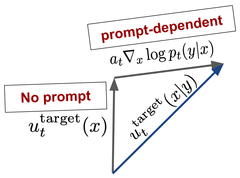
Reparameterization: Velocity Field → Score Function
\[a_t = \left(\beta_t^2 \frac{\dot{\alpha}_t}{\alpha_t} - \dot{\beta}_t \beta_t\right), \qquad b_t = \frac{\dot{\alpha}_t}{\alpha_t}\]
\[ \begin{align} u_t^{\text{target}}(x|z) &= a_t \nabla \log p_t(x|z) + b_t x \\ u_t^{\text{target}}(x) &= a_t \nabla \log p_t(x) + b_t x \end{align} \]
Denoising Score Matching for Gaussian Prob. Path
\[\nabla \log p_t(x|z) = -\frac{x - \alpha_t z}{\beta_t^2}\]
\[\epsilon \sim \mathcal{N}(0, I_d) \quad \Rightarrow \quad x = \alpha_t z + \beta_t \epsilon \sim \mathcal{N}(\alpha_t z,\, \beta_t^2 I_d)\]
\[ \begin{align} \mathcal{L}_{\text{dsm}}(\theta) &= \mathbb{E}_{t \sim \text{Unif},\, z \sim p_{\text{data}},\, x \sim p_t(\cdot|z)}\!\left[\left\|s_t^\theta(x) + \frac{x - \alpha_t z}{\beta_t^2}\right\|^2\right] \\ &= \mathbb{E}_{t \sim \text{Unif},\, z \sim p_{\text{data}},\, \epsilon \sim \mathcal{N}(0,I_d)}\!\left[\left\|s_t^\theta(\alpha_t z + \beta_t \epsilon) + \frac{\epsilon}{\beta_t}\right\|^2\right] \end{align} \]
Note what the network does: It needs to predict the noise that was used to corrupt the data point! (DENOISING diffusion models)
Fokker-Planck Equation
Randomly initialized SDE
Given: \(\quad X_0 \sim p_{\text{init}}, \qquad \mathrm{d}X_t = u_t(X_t)\mathrm{d}t + \sigma_t\mathrm{d}W_t\)
Follow probability path:
\[X_t \sim p_t \qquad (0 \le t \le 1)\]
Marginals are \(p_t\)
\(\Longleftrightarrow\) equivalent
Fokker-Planck equation holds
\[\frac{\mathrm{d}}{\mathrm{d}t}p_t(x) = \underbrace{-\operatorname{div}(p_t u_t)(x)}_{\color{#a30000}{\small\textit{Continuity equation}}} + \underbrace{\frac{\sigma_t^2}{2}\Delta p_t(x)}_{\color{#a30000}{\small\textit{Heat equation}}}\]
Fokker-Planck Equation
\[\underbrace{\frac{\mathrm{d}}{\mathrm{d}t}p_t(x)}_{\color{#a30000}{\small\textit{Change of prob. mass at } x}} = \underbrace{-\operatorname{div}(p_t u_t)(x)}_{\color{#a30000}{\small\textit{Mass conservation}}} + \underbrace{\frac{\sigma_t^2}{2}\Delta p_t(x)}_{\color{#a30000}{\small\textit{Heat dispersion}}}\]
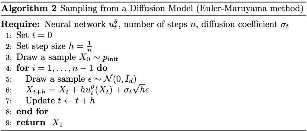
Stochastic Sampling of Diffusion Models
Choose noise level \(\sigma_t\). By “SDE extension trick”, we can sample from:
\[\mathrm{d}X_t = \left[{\color{#1a6faf}{u_t^{\text{target}}(X_t)}} + {\color{#2a9a2a}{\frac{\sigma_t^2}{2}\nabla \log p_t(X_t)}}\right]\mathrm{d}t + \sigma_t\mathrm{d}W_t\]
For Gaussian probability paths, we can express this solely in terms of the score:
\[\mathrm{d}X_t = \left[\left(a_t + \frac{\sigma_t^2}{2}\right)\nabla \log p_t(X_t) + b_t X_t\right]\mathrm{d}t + \sigma_t\mathrm{d}W_t\]
Plugin score network:
\[\mathrm{d}X_t = \left[\left(a_t + \frac{\sigma_t^2}{2}\right)s_t^\theta(X_t) + b_t X_t\right]\mathrm{d}t + \sigma_t\mathrm{d}W_t\]
Why Would We Want Stochastic/SDE Dynamics?
In theory: All diffusion coefficients lead to the same result (sample from data distribution).
In practice:
- Training error: Neural network has not perfectly learnt the marginal vector field/score.
- Simulation error: We need to simulate SDE/ODE leading to discretization error.
Downstream applications: Fine-tuning, inference-time optimization, etc. might require stochastic evolution
Good news: ODE sampling often leads to the best results. Therefore, SDE sampling is an option, not a must!
Image source: Scaling Rectified Flow Transformers for High-Resolution Image Synthesis [1]

A swamp ogre with a pearl earring by Johannes Vermeer
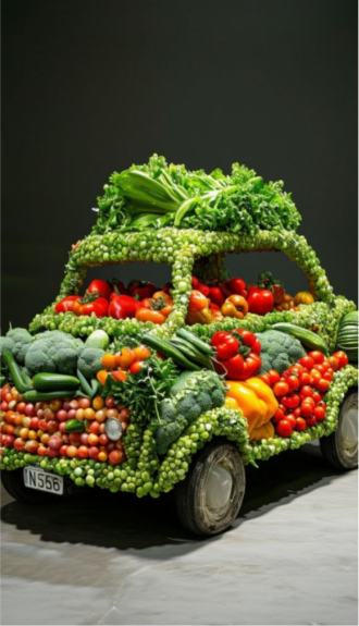
A car made out of vegetables.

heat death of the universe, line art
Unguided: Generate an image.
Guided: Generate an image of a cat baking a cake.
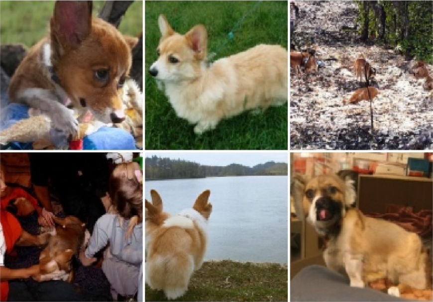
Vanilla Guided Sampling
Vanilla Guidance leads to suboptimal results
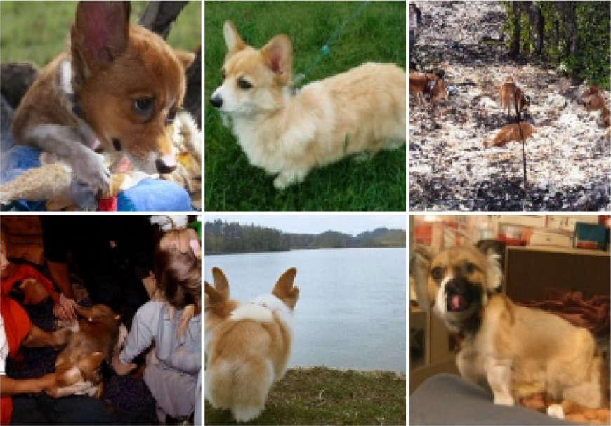
Prompt: “Corgi dog”
These images do not fit well to the prompt and they have errors!
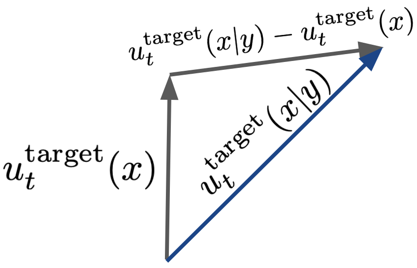
Intuition: Classifier Guidance
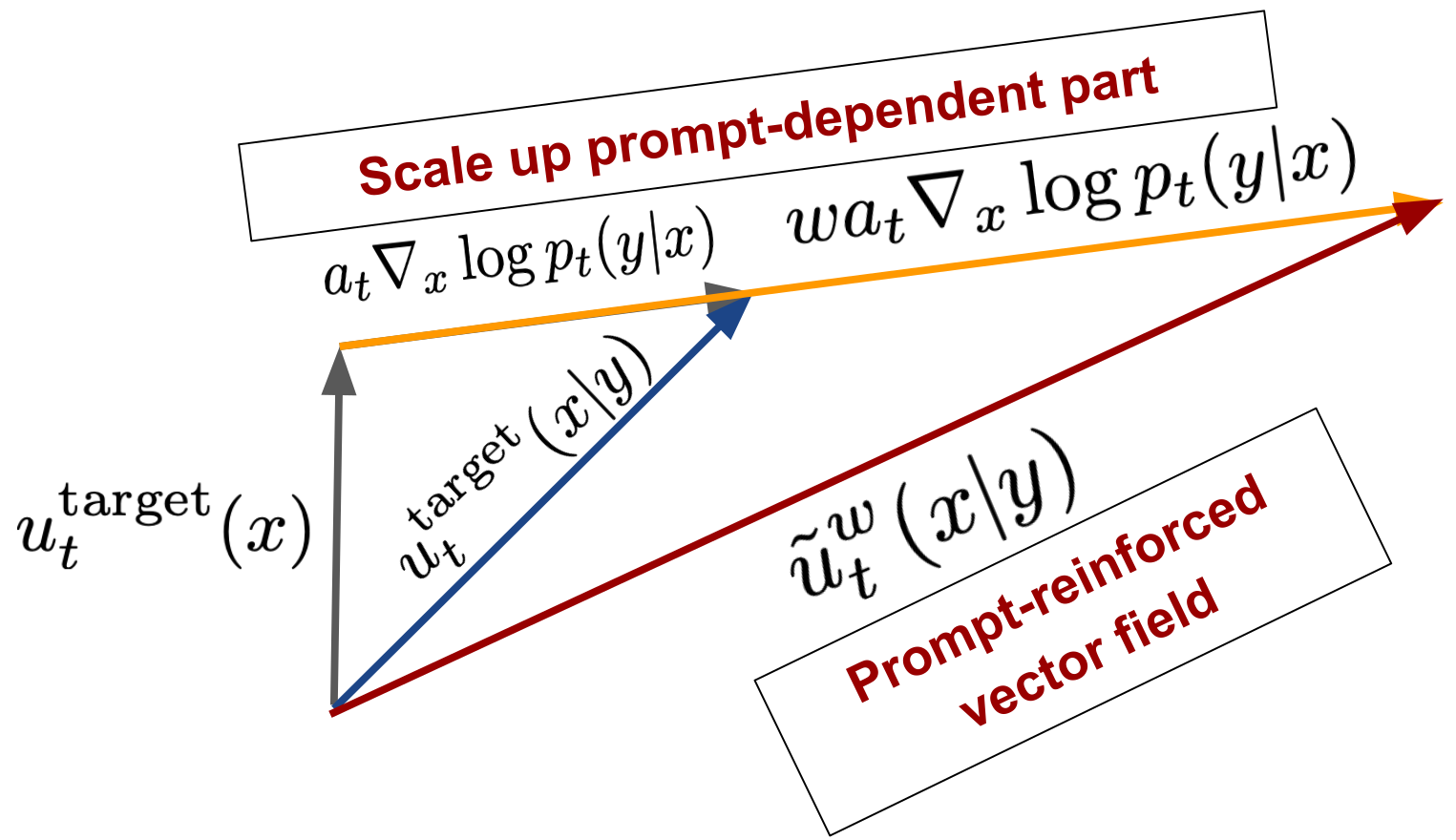
Classifier-Free Guidance
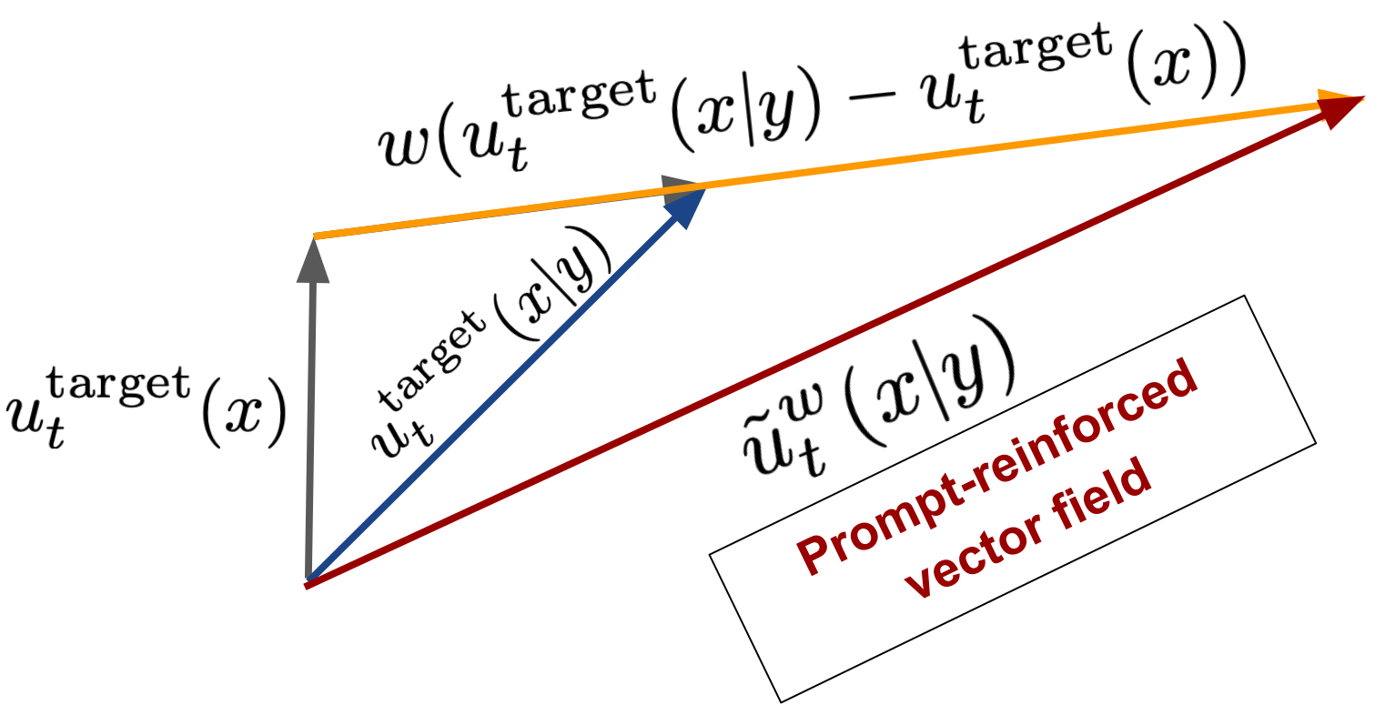
Classifier-free guidance training: Account for empty token \(\varnothing\)
Sampling with Classifier-Free Guidance
Simply is the same as before but we use the weighted vector field:
\[u_t^{\theta,w}(x) = (1-w)u_t^\theta(x|\varnothing) + wu_t^\theta(x|y)\]
Example: Classifier-Free Guidance
w=1.0
w=4.0
Example: Classifier-Free Guidance