$$ % Define your custom commands here \newcommand{\bmat}[1]{\begin{bmatrix}#1\end{bmatrix}} \newcommand{\E}{\mathbb{E}} \newcommand{\P}{\mathbb{P}} \newcommand{\S}{\mathbb{S}} \newcommand{\R}{\mathbb{R}} \newcommand{\S}{\mathbb{S}} \newcommand{\norm}[2]{\|{#1}\|_{{}_{#2}}} \newcommand{\pd}[2]{\frac{\partial #1}{\partial #2}} \newcommand{\pdd}[2]{\frac{\partial^2 #1}{\partial #2^2}} \newcommand{\vectornorm}[1]{\left|\left|#1\right|\right|} \newcommand{\abs}[1]{\left|{#1}\right|} \newcommand{\mbf}[1]{\mathbf{#1}} \newcommand{\mc}[1]{\mathcal{#1}} \newcommand{\bm}[1]{\boldsymbol{#1}} \newcommand{\nicefrac}[2]{{}^{#1}\!/_{\!#2}} \newcommand{\argmin}{\operatorname*{arg\,min}} \newcommand{\argmax}{\operatorname*{arg\,max}} \newcommand{\dd}{\operatorname{d}\!} $$

Neural Operators and U-Net

Notes adapted from UNet Tutorial in JAX Machine Learning & Simulation

Notes adapted from MIT OpenCourseWare Adjoint Differentiation of ODE Solutions

A simple implementation of a hierarchical convolutional neural network in JAX; used to learn a solver to a $1$D Poisson equation. \[ \frac{\dd^2 u}{\dd x^2} = -f(x), \quad x \in (0, L), \quad u(0) = u(L) = 0. \] The Poisson equation (together with homogeneous Dirichlet boundary conditions) maps a force field $f(x)$ to the displacement $u(x)$ of a thin string.

The U-Net $f_\theta$ is trained to map $f(x) \mapsto u(x)$.
In this concrete scenario, the forcing functions will have a discontinuity: \[ f(x) = \begin{cases} 1 & x \in [\ell_0, \ell_1] \\ 0 & \text{otherwise} \end{cases} \] with $\ell_0 \propto \mathcal{U}\left(\nicefrac{L}{5}, \nicefrac{2L}{5}\right)$ and $\ell_1 \propto \mathcal{U}\left(\nicefrac{3L}{5}, \nicefrac{4L}{5}\right)$.
We will draw $P = 1,000$ forcing functions and then discretize them on a grid of $N = 32$ interior nodes.
A reference solution is computed by a direct linear solver applied to the three-point discretization.
With a $4:1$ train/test split, the U-Net is trained on MSE error on batch size of $\abs{\mc{B}} = 32$ for $100$ epochs.

Dataset Generation

Discretize the interval $(0, L)$ at $N+2$ equally-spaced points ($2$ gridpoints at the endpoints, remaining $N$ in the interior of the domain)
Define the grid spacing as $h = \nicefrac{L}{N}$.
The forcing function is discretized as \[ f_j = f(x_j), \quad j = 1, \dots, N. \]
The solution is discretized as \[ u_j = u(x_j), \quad j = 1, \dots, N. \]
The second-order central difference approximation to the second derivative is \[ \frac{\dd^2 u}{\dd x^2} \approx \frac{u_{j-1} - 2u_j + u_{j+1}}{h^2}. \]
- This follows from defining the first-order central difference as \[ \frac{\dd u}{\dd x} \approx \frac{u_{j+\nicefrac{1}{2}} - u_{j-\nicefrac{1}{2}}}{h}. \]
- Iterating this a second time \[ \frac{\dd^2 u}{\dd x^2} \approx \frac{\frac{u_{j+1} - u_j}{h} - \frac{u_j - u_{j-1}}{h}}{h} = \frac{u_{j-1} - 2u_j + u_{j+1}}{h^2}. \]
The boundary conditions are \[ u_0 = u_{N+1} = 0. \]
Substituting these into the Poisson equation yields a linear system of equations for the interior nodes: \[ -u_{j-1} + 2u_j - u_{j+1} = h^2 f_j, \quad j = 1, \dots, N. \]
This yields a linear system of the form \[ \bm{A} \bm{u} = -h^2 \bm{f}, \] where $\bm{A}$ is the following tridiagonal matrix: \[ \bm{A} = \begin{pmatrix} 2 & -1 & 0 & \dots & 0 \\ -1 & 2 & -1 & \dots & 0 \\ 0 & -1 & 2 & \dots & 0 \\ \vdots & \vdots & \vdots & \ddots & \vdots \\ 0 & 0 & 0 & -1 & 2 \end{pmatrix}. \]
Solving this system yields the (discretized) solution $\bm{u}$ to a given (discretized) forcing function $\bm{f}$.

Dataset Generation

import jax
import jax.numpy as jnp

NUM_POINTS = 32         # N
NUM_SAMPLES = 1000      # P
DOMAIN_EXTENT = 5.0     # L

# Interior grid (excludes the two Dirichlet boundary points)
grid = jnp.linspace(0, DOMAIN_EXTENT, NUM_POINTS + 2)[1:-1]
dx = grid[1] - grid[0]

# Second-order finite-difference matrix  A ≈ d²/dx²
_A = (
    jnp.diag(jnp.ones(NUM_POINTS - 1), -1)
    - 2 * jnp.diag(jnp.ones(NUM_POINTS), 0)
    + jnp.diag(jnp.ones(NUM_POINTS - 1), 1)
) / dx**2


def solve_poisson(f: jax.Array) -> jax.Array:
    """Solve  A u = -f  for u given a force field f on the interior grid."""
    return jnp.linalg.solve(_A, -f)


def create_discontinuity(key: jax.Array) -> jax.Array:
    """
    Generate a random box-function force field on the interior grid.
    The active interval is drawn uniformly from [0.2L, 0.4L] x [0.6L, 0.8L].
    """
    limit_1_key, limit_2_key = jax.random.split(key)
    lower_limit = jax.random.uniform(
        limit_1_key, (), minval=0.2 * DOMAIN_EXTENT, maxval=0.4 * DOMAIN_EXTENT
    )
    upper_limit = jax.random.uniform(
        limit_2_key, (), minval=0.6 * DOMAIN_EXTENT, maxval=0.8 * DOMAIN_EXTENT
    )
    return jnp.where((grid >= lower_limit) & (grid <= upper_limit), 1.0, 0.0)


def generate_dataset(
    num_samples: int = NUM_SAMPLES,
    seed: int = 0,
) -> tuple[jax.Array, jax.Array]:
    """
    Generate (force_fields, displacement_fields) each of shape
    (num_samples, 1, NUM_POINTS) — channel-first, ready for Conv1d.

    Returns
    -------
    force_fields : jax.Array, shape (N, 1, NUM_POINTS)
    displacement_fields : jax.Array, shape (N, 1, NUM_POINTS)
    """
    primary_key = jax.random.PRNGKey(seed)
    keys = jax.random.split(primary_key, num_samples)

    force_fields = jax.vmap(create_discontinuity)(keys)          # (N, P)
    displacement_fields = jax.vmap(solve_poisson)(force_fields)  # (N, P)

    # Add singleton channel axis → (N, 1, P)
    force_fields = force_fields[:, None, :]
    displacement_fields = displacement_fields[:, None, :]

    return force_fields, displacement_fields


def train_test_split(
    force_fields: jax.Array,
    displacement_fields: jax.Array,
    train_fraction: float = 0.8,
) -> tuple[jax.Array, jax.Array, jax.Array, jax.Array]:
    """
    Split arrays into train / test sets.

    Returns
    -------
    train_x, test_x, train_y, test_y
    """
    split = int(force_fields.shape[0] * train_fraction)
    return (
        force_fields[:split],
        force_fields[split:],
        displacement_fields[:split],
        displacement_fields[split:],
    )

U-Net Implementation

Original UNet schematic by Ronneberger et al. (2015) (our concrete implementation deviates from this)

Modifications from the classical U-Net

Use linear convolution for downscaling instead of max-pooling
Downscaling and upscaling are $3 \times 3$ convolutions with stride $2$ (instead of $2 \times 2$)
“Same” padding to never have issues with spatial sizes
No normalization layers for simplicity
Variable number levels (here we will use two)

U-Net neural operator implemented with Equinox

"""
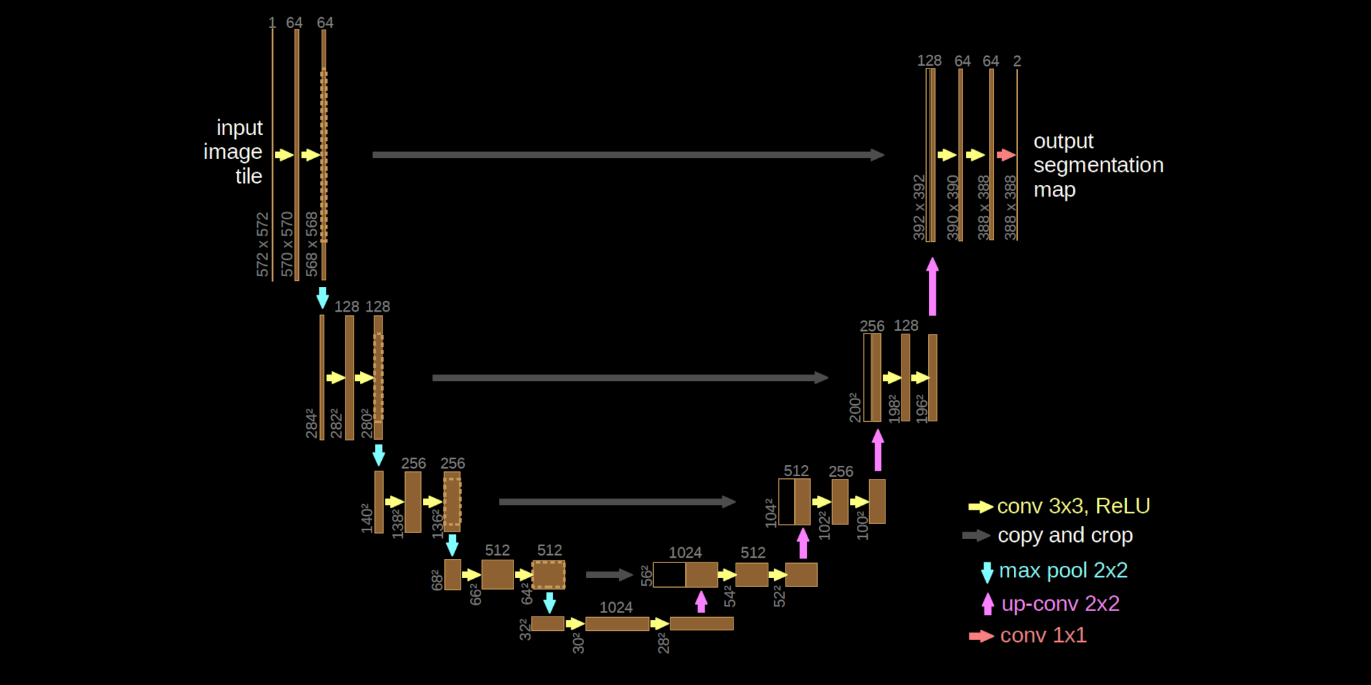
U-Net neural operator implemented with Equinox.

Architecture:
  - Lifting DoubleConv
  - Encoder: stride-2 Conv downsampling + DoubleConv at each level
  - Decoder: ConvTranspose upsampling + skip-connection concat + DoubleConv
  - 1x1 Conv projection to output channels
"""

import jax
import jax.numpy as jnp
import jax.tree_util as jtu
import equinox as eqx
from typing import Callable


class DoubleConv(eqx.Module):
    conv_1: eqx.nn.Conv
    conv_2: eqx.nn.Conv
    activation: Callable

    def __init__(
        self,
        num_spatial_dims: int,
        in_channels: int,
        out_channels: int,
        activation: Callable,
        *,
        key,
    ):
        c_1_key, c_2_key = jax.random.split(key)
        self.conv_1 = eqx.nn.Conv(
            num_spatial_dims,
            in_channels,
            out_channels,
            kernel_size=3,
            padding=1,
            key=c_1_key,
        )
        self.conv_2 = eqx.nn.Conv(
            num_spatial_dims,
            out_channels,
            out_channels,
            kernel_size=3,
            padding=1,
            key=c_2_key,
        )
        self.activation = activation

    def __call__(self, x: jax.Array) -> jax.Array:
        x = self.activation(self.conv_1(x))
        x = self.activation(self.conv_2(x))
        return x


class UNet(eqx.Module):
    lifting: DoubleConv
    down_sampling_blocks: list[eqx.nn.Conv]
    left_arc_blocks: list[DoubleConv]
    right_arc_blocks: list[DoubleConv]
    up_sampling_blocks: list[eqx.nn.ConvTranspose]
    projection: eqx.nn.Conv

    def __init__(
        self,
        num_spatial_dims: int,
        in_channels: int,
        out_channels: int,
        hidden_channels: int,
        num_levels: int,
        activation: Callable,
        *,
        key,
    ):
        key, lifting_key, projection_key = jax.random.split(key, 3)

        self.lifting = DoubleConv(
            num_spatial_dims,
            in_channels,
            hidden_channels,
            activation,
            key=lifting_key,
        )
        self.projection = eqx.nn.Conv(
            num_spatial_dims,
            hidden_channels,
            out_channels,
            kernel_size=1,
            key=projection_key,
        )

        # Channel counts at each level: [C, 2C, 4C, ...]
        channel_list = [hidden_channels * 2**i for i in range(num_levels + 1)]

        self.down_sampling_blocks = []
        self.left_arc_blocks = []
        self.right_arc_blocks = []
        self.up_sampling_blocks = []

        for upper_ch, lower_ch in zip(channel_list[:-1], channel_list[1:]):
            key, down_key, left_key, right_key, up_key = jax.random.split(key, 5)

            self.down_sampling_blocks.append(
                eqx.nn.Conv(
                    num_spatial_dims,
                    upper_ch,
                    upper_ch,
                    kernel_size=3,
                    stride=2,
                    padding=1,
                    key=down_key,
                )
            )
            self.left_arc_blocks.append(
                DoubleConv(num_spatial_dims, upper_ch, lower_ch, activation, key=left_key)
            )
            self.right_arc_blocks.append(
                DoubleConv(num_spatial_dims, lower_ch, upper_ch, activation, key=right_key)
            )
            self.up_sampling_blocks.append(
                eqx.nn.ConvTranspose(
                    num_spatial_dims,
                    lower_ch,
                    upper_ch,
                    kernel_size=3,
                    stride=2,
                    padding=1,
                    output_padding=1,
                    key=up_key,
                )
            )

    def __call__(self, x: jax.Array) -> jax.Array:
        x = self.lifting(x)
        x_skips = []

        # Encoder (left arc)
        for down, left in zip(self.down_sampling_blocks, self.left_arc_blocks):
            x_skips.append(x)
            x = down(x)
            x = left(x)

        # Decoder (right arc)
        for right, up in zip(
            reversed(self.right_arc_blocks), reversed(self.up_sampling_blocks)
        ):
            x = up(x)
            # Equinox operates without a batch axis; channels are at axis 0
            x = jnp.concatenate([x, x_skips.pop()], axis=0)
            x = right(x)

        return self.projection(x)


def count_parameters(model: eqx.Module) -> int:
    """Return the total number of trainable scalar parameters."""
    return sum(p.size for p in jtu.tree_leaves(eqx.filter(model, eqx.is_array)))

Training and Results

Training and results

# ---------------------------------------------------------------------------
# Hyper-parameters
# ---------------------------------------------------------------------------
HIDDEN_CHANNELS = 32
NUM_LEVELS = 2
LEARNING_RATE = 3e-4
NUM_EPOCHS = 100
BATCH_SIZE = 32
SEED_DATA = 0
SEED_MODEL = 0
SEED_SHUFFLE = 151


# ---------------------------------------------------------------------------
# Helpers
# ---------------------------------------------------------------------------
def dataloader(data, *, batch_size: int, key):
    """Mini-batch generator over a PyTree / tuple of arrays."""
    n_samples_list = [a.shape[0] for a in jtu.tree_leaves(data)]
    if not all(n == n_samples_list[0] for n in n_samples_list):
        raise ValueError("All arrays must have the same leading (sample) dimension.")
    n_samples = n_samples_list[0]
    n_batches = int(jnp.ceil(n_samples / batch_size))
    permutation = jax.random.permutation(key, n_samples)

    for batch_id in range(n_batches):
        start = batch_id * batch_size
        end = min((batch_id + 1) * batch_size, n_samples)
        indices = permutation[start:end]
        yield jtu.tree_map(lambda a: a[indices], data)


def normalized_l2_norm(pred: jax.Array, ref: jax.Array) -> jax.Array:
    """Per-sample normalised L2 error: ||pred - ref|| / ||ref||."""
    return jnp.linalg.norm(pred - ref) / jnp.linalg.norm(ref)


# ---------------------------------------------------------------------------
# Loss and update step
# ---------------------------------------------------------------------------
def loss_fn(model, x, y):
    y_pred = jax.vmap(model)(x)
    return jnp.mean(jnp.square(y_pred - y))


def make_update_fn(optimizer):
    """Closes over optimizer so filter_jit doesn't see it as a traced value."""
    @eqx.filter_jit
    def update_fn(model, opt_state, x, y):
        loss, grad = eqx.filter_value_and_grad(loss_fn)(model, x, y)
        updates, new_state = optimizer.update(grad, opt_state, model)
        new_model = eqx.apply_updates(model, updates)
        return new_model, new_state, loss
    return update_fn


# ---------------------------------------------------------------------------
# Main
# ---------------------------------------------------------------------------
def main():
    # -- Dataset -----------------------------------------------------------
    print("Generating dataset …")
    force_fields, displacement_fields = generate_dataset(seed=SEED_DATA)
    train_x, test_x, train_y, test_y = train_test_split(force_fields, displacement_fields)
    print(f"  train: {train_x.shape}  test: {test_x.shape}")

    # -- Model -------------------------------------------------------------
    model = UNet(
        num_spatial_dims=1,
        in_channels=1,
        out_channels=1,
        hidden_channels=HIDDEN_CHANNELS,
        num_levels=NUM_LEVELS,
        activation=jax.nn.relu,
        key=jax.random.PRNGKey(SEED_MODEL),
    )
    print(f"  parameters: {count_parameters(model):,}")

    optimizer = optax.adam(LEARNING_RATE)
    opt_state = optimizer.init(eqx.filter(model, eqx.is_array))
    update_fn = make_update_fn(optimizer)

    # -- Training loop -----------------------------------------------------
    loss_history = []
    shuffle_key = jax.random.PRNGKey(SEED_SHUFFLE)

    for epoch in tqdm(range(NUM_EPOCHS), desc="epochs"):
        shuffle_key, subkey = jax.random.split(shuffle_key)
        for batch in dataloader((train_x, train_y), batch_size=BATCH_SIZE, key=subkey):
            model, opt_state, loss = update_fn(model, opt_state, *batch)
            loss_history.append(float(loss))

    # -- Evaluation --------------------------------------------------------
    test_predictions = jax.vmap(model)(test_x)
    test_errors = jax.vmap(normalized_l2_norm)(test_predictions, test_y)

Ordinary Differential Equations (ODEs)

Initial Value Problem \[ \begin{aligned} \frac{\dd u}{\dd t}(t) &= f(t, u(t), \theta) \\ u(t_0) &= u_0 \end{aligned} \]
How do we solve an ODE?

Toy Example: Free falling ball

ODE with state $u(t) = \bmat{z(t) & v(t)}^\top$ \[ \begin{aligned} \dd z(t) &= v(t) \dd t && z(t=t_0) = z_0 = 5 \text{ m}\\ \dd v(t) &= -g \dd t && v(t=t_0) = v_0 = -\nicefrac{1}{10} \text{ m/s} \end{aligned} \]
Analytical solution (available in this case) \[ \begin{aligned} z(t) &= z_0 + v_0 (t-t_0) - \frac{1}{2} g (t-t_0)^2 \\ v(t) &= v_0 - g (t-t_0) \end{aligned} \]

More generally, we would have a numerical solver, the simplest of which is the Euler method \[ \begin{aligned} u_{n+1} &= u_n + \Delta t f(t_n, u_n, p), \\ t_n &= t_0 + n \Delta t \end{aligned} \]
There are tons of more sophisticated methods.

Sensitivities

Different methods for performing sensitivity analysis of ODEs

Two main ways of differentiating through an ODE
- Discrete sensitivity analysis (autodiff on solver operations)
  - “Exact gradient approximation” or “discretize-then-differentiate”
- Continuous sensitivity analysis (custom rules)
  - “Approximation of the exact gradient” or “differentiate-then-discretize”
Two modes each (forward/tangent and reverse/adjoint)
- Best choice depends on the number of states/parameters and system properties.

What are sensitivities or derivatives good for?

Sensitivity analysis
- How sensitive is the solution to changes in the initial conditions (ICs) and/or parameters?
Parameter estimation
- What parameters match the observed data?
Control
- How can I drive the solution to a certain final state?

Toy Example: Parameter Estimation

For the free-falling ball example, let us consider loss function \[ \mc{J}(z; g) = \frac{1}{2} \left(z(T; g) - z_{\text{obs}}\right)^2, \] where $z(T; g)$ is the analytical solution and $z_{\text{obs}}$ is the observed position at time $T$.
We want to take the derivative of $\mc{J}$ with respect to $g$
- By the chain rule, this requires, in turn, that we compute the derivative of $z(T; g)$ with respect to $g$.
Since we know the analytical solution, this computation is easy. \[ \pd{z(T; g)}{g} = \pd{}{g} \left( z_0 + v_0 (T-t_0) - \frac{1}{2} g (T-t_0)^2 \right) = -\frac{1}{2} (T-t_0)^2 \]

In general, we have a loss functional $\mc{J}(u; p)$, for example, \[ \begin{aligned} \mc{J}(u; p) &= \int_{t_0}^T r(u; p) \dd t, \\ r(u; p) &= u^\top Q u. \end{aligned} \]
We want to compute its sensitivity $\frac{\dd \mc{J}}{\dd p}$.

Total Derivative

Let’s compute the total derivative of the loss functional with respect to the parameters.

\[ \frac{\dd \mc{J}}{\dd p} = \int_{t_0}^T \frac{\dd r}{\dd p} \dd t = \int_{t_0}^T \left( \frac{\partial r}{\partial p} + \frac{\partial r}{\partial u} \frac{\dd u}{\dd p}\right) \dd t, \tag{1}\] where $\pd{r}{p} \in \R^{1 \times n_p}$, $\pd{r}{u} \in \R^{1 \times n_u}$ and $\pd{u}{p} \in \R^{n_u \times n_p}$.

The term $\pd{u}{p}$ is difficult to compute, since it requires solving an ODE for each parameter.
Two choices:
1. Forward sensitivity
2. Adjoint or backward sensitivity

Forward Sensitivity Analysis

The goal is to compute the sensitivity matrix (Jacobian) of the state with respect to the parameters: \[ \frac{\dd u}{\dd p} = \begin{pmatrix} | & & | \\ \pd{u}{p_1} & \dots & \pd{u}{p_m} \\ | & & | \end{pmatrix} \in \R^{n_u \times n_p} \]

Consider the Initial Value Problem (IVP): \[ \begin{cases} \frac{\dd u}{\dd t} = f(t, u, p) \\ u(0) = u_0 \end{cases} \]

To find how the solution $u$ changes with respect to a parameter $p_i$, we implicitly differentiate the ODE: \[ \frac{\dd}{\dd p_i} \left( \frac{\dd u}{\dd t} \right) = \pd{}{p_i} f(t, u, p) \]

By swapping the order of differentiation $\left(\frac{\dd}{\dd p_i} \frac{\dd}{\dd t} \to \frac{\dd}{\dd t} \frac{\dd}{\dd p_i}\right)$ and applying the chain rule to the right-hand side: \[ \frac{\dd}{\dd t} \left( \pd{u}{p_i} \right) = \pd{f}{u} \pd{u}{p_i} + \pd{f}{p_i} \]

Let $s_i = \pd{u}{p_i}$ be the sensitivity of the state with respect to parameter $p_i$. This yields a new IVP for each sensitivity vector: \[ \begin{cases} \frac{\dd s_i}{\dd t} = \pd{f}{u} s_i + \pd{f}{p_i} \\ s_i(t_0) = \pd{u_0}{p_i} \end{cases} \]

Summary:

Build the Jacobian $\pd{u}{p}$ by solving the $n_u \times n_p$ sensitivity equations alongside the original ODE.
Plug the sensitivities into the total derivative integral in Equation 1 and solve by quadrature.
Scalability: This method scales linearly with the number of parameters $n_p$!

Adjoint Sensitivity Analysis

We aim to solve the following constrained optimization problem: \[ \begin{aligned} \min_p \quad & \mc{J}(u; p) \\ \text{subj. to} \quad & \frac{\dd u}{\dd t} = f(u, t, p) \end{aligned} \] This is a dynamic equality constrained optimization problem. We can define the Lagrangian: \[ L(u, \lambda; p) = \mc{J}(u; p) + \int_{t_0}^T \lambda^\top \left( f - \frac{\dd u}{\dd t} \right) \dd t, \] where $\lambda$ is a continuous Lagrange multiplier with $\lambda(t) \in \R^{n_u}$. Using the integral form of $\mc{J}$ from Equation 1: \[ L = \int_{t_0}^T \left[ r(u; p) + \lambda^\top(t) \left( f - \frac{\dd u}{\dd t} \right) \right] \dd t \] Differentiating with respect to $p$: \[ \frac{\dd L}{\dd p} = \int_{t_0}^T \left[ \pd{r}{p} + \pd{r}{u} \frac{\dd u}{\dd p} + \lambda^\top(t) \left( \pd{f}{p} + \pd{f}{u} \frac{\dd u}{\dd p} - \frac{\dd}{\dd t} \frac{\dd u}{\dd p} \right) \right] \dd t. \] Here, the terms $\frac{\dd u}{\dd p}$ are difficult to compute. Rearranging the terms: \[ \frac{\dd L}{\dd p} = \int_{t_0}^T \left[ \pd{r}{p} + \lambda^\top \pd{f}{p} + \underbrace{\left( \pd{r}{u} + \lambda^\top \pd{f}{u} - \lambda^\top \frac{\dd}{\dd t} \right)}_{\text{make zero}} \frac{\dd u}{\dd p} \right] \dd t \tag{2}\]

Integration-by-parts

We can integrate the term $\int_{t_0}^T \lambda^\top \frac{\dd}{\dd t} \frac{\dd u}{\dd p} \dd t$ by parts:

\[ \begin{aligned} \int_{t_0}^T -\lambda^\top \frac{\dd}{\dd t} \frac{\dd u}{\dd p} \dd t &= \left[ -\lambda^\top \frac{\dd u}{\dd p} \right]_{t_0}^T + \int_{t_0}^T \frac{\dd \lambda}{\dd t}^\top \frac{\dd u}{\dd p} \dd t \\ &= \lambda^\top(t_0) \frac{\dd u}{\dd p}(t_0) - \lambda^\top(T) \frac{\dd u}{\dd p}(T) + \int_{t_0}^T \frac{\dd \lambda}{\dd t}^\top \frac{\dd u}{\dd p} \dd t \end{aligned} \]

Substituting the result from the integration-by-parts into Equation 2 gives

\[ \frac{\dd L}{\dd p} = \int_{t_0}^T \left[ \pd{r}{p} + \lambda^\top \pd{f}{p} + \underbrace{\left( \pd{r}{u} + \lambda^\top \pd{f}{u} + \frac{\dd \lambda}{\dd t}^\top \right)}_{\text{make zero}} \frac{\dd u}{\dd p} \right] \dd t + \lambda^\top(t_0) \frac{\dd u}{\dd p}(t_0) - \underbrace{\lambda(T)^\top}_{\text{make zero}} \frac{\dd u}{\dd p}(T). \]

Hence, we choose the Lagrange multiplier $\lambda$ such that \[ \pd{r}{u}^\top + \lambda^\top \pd{f}{u} + \frac{\dd \lambda}{\dd t}^\top = 0, \quad \lambda(T) = 0 \] Taking the transpose yields \[ \begin{cases} \dot{\lambda} = -f_u^\top \lambda - r_u^\top \\ \lambda(T) = 0 \end{cases} \]

This is a terminal value problem that must be solved backwards in time. With this choice of $\lambda$, the total derivative simplifies to: \[ \frac{\dd \mc{J}}{\dd p} = \frac{\dd \mc{L}}{\dd p} = \int_{t_0}^T \left[ \pd{r}{p} + \lambda^\top \pd{f}{p} \right] \dd t + \lambda^\top(t_0) \pd{u}{p}(t_0) \]

Numerical Strategy:

Solve forward: $\dot{u} = f(u, t, p)$ with $u(t_0) = u_0$ to obtain $u(t)$ for $t \in [t_0, T]$.
Solve backward: $\dot{\lambda} = -\pd{f}{u}^\top \lambda - \pd{r}{u}^\top$ with $\lambda(T) = 0$ to obtain $\lambda(t)$.
Evaluate: Compute the gradient using the quadrature: \[ \frac{\dd \mc{J}}{\dd p} = \int_{t_0}^T \left[ \pd{r}{p} + \lambda^\top \pd{f}{p} \right] \dd t + \lambda^\top(t_0) \pd{u}{p}(t_0) \]

Scalability: This method scales constantly with the number of parameters $n_p$!

Tips and Tricks

To avoid storing the continuous solution $u(t)$, solve it once forward to obtain $u(T)$, then solve the $\dot{u}$ ODE in lock-step with the $\dot{\lambda}$ ODE starting from this final solution (Doesn’t always work, especially for chaotic systems).
Quadrature as an ODE \[ F(T) = \int_{t_0}^T f(t) \dd t \quad ; \quad \dot{w}(t) = f(t), \quad w(t_0) = 0 \] \[ w(t+n \Delta t) \approx w(t) + \Delta t \sum_{k=0}^n f(t+k \Delta t) \]
Adjoint Augmented Dynamics For the case where we want to compute the derivative of the loss with respect to parameters: \[ \begin{aligned} \dot{w} &= g_p + \lambda^\top f_p, && w(T) = 0 \\ \dot{\lambda} &= -f_u^\top \lambda - g_u^\top, && \lambda(T) = 0 \\ \dot{u} &= f(t, u, p), && u(T) = u_{\text{end}} \end{aligned} \] $w$ is the derivative you want!

Learning the gravitational acceleration with Euler method

import jax
import jax.numpy as jnp

z0 = jnp.array(5.0)
v0 = jnp.array(0.1)
p_true = jnp.array(3.70)
p = jnp.array(10.56)

u0 = jnp.array([z0, v0])
tspan = jnp.array([0.0, 1.0])
dt = 0.001
n_steps = int((tspan[1] - tspan[0]) // dt)

eta = 0.25

z_cf = jax.jit(lambda t, p: z0 + v0 * t - 0.5 * p * t ** 2)
v_cf = jax.jit(lambda t, p: v0 - p * t)

def freefall(u, t, p):
    z, v = u
    dzdt = v
    dvdt = -p
    return jnp.array([dzdt, dvdt])

def euler_step(f, u, t, dt, p):
    return u + dt * f(u, t, p)

def rollout(
    stepper_fn, 
    n,
    *,
    include_init=False,
):
    def scan_fn(u, t):  # State x Time(and/or Control)->New_State x Observation
        u_next = stepper_fn(u, t)
        obs = dt * 1/2 * (u_next[0] - z_cf(t, p_true)) ** 2
        # obs = jnp.abs(u_next[0] - z_cf(t, p_true)) * dt
        # u_next_true = jnp.array([z_cf(t, p_true), v_cf(t, p_true)])
        # state_error = u_next - u_next_true
        # obs = dt * 1/2 * jnp.dot(state_error, state_error)
        return u_next, (u_next, obs)

    def rollout_fn(init):
        xs = jnp.linspace(tspan[0], tspan[1], n)
        _, history = jax.lax.scan(
            scan_fn,    # Euler step
            init,       # Initial state
            xs,         # tspan, (could also include Forcing trajectory)
            length=n,   # Number of steps
        )

        if include_init:
            init_obs = (u0, 0.0)
            return (jnp.concatenate(
                [jnp.expand_dims(init_obs[0], axis=0), history[0]], 
                axis=0), 
                jnp.concatenate(
                [jnp.expand_dims(init_obs[1], axis=0), history[1]],
                axis=0),
            )

        return history
    return rollout_fn

trj = lambda p: rollout(
        lambda u, t: euler_step(freefall, u, t, dt, p), 
        n_steps, include_init=True
    )

@jax.jit
@jax.value_and_grad
def loss(p):
    return jnp.sum(trj(p)(u0)[1])

N = int(2 ** 10)
for i in range(N):
    l, grad = loss(p)
    p -= eta * grad
    if i % (2**(jnp.log2(N)//2)) == 0 or i == N-1:
        print('i={:3d}, loss={:.3e}, grad={:.4f}, p={:.4f}'.format(i, l, grad, p))

Learning the gravitational acceleration with the adjoint method

import jax 
from jax import numpy as jnp

z0 = 5.0
v0 = 0.1
g_true = 9.802
g = 20.0
p_true = jnp.array(g_true)
p = jnp.array(g)

u0 = jnp.array([z0, v0])
tspan = jnp.array([0.0, 1.0])
dt = 0.005
n_steps = int((tspan[1] - tspan[0]) // dt)

eta = 1.0

# %% 
z_cf = jax.jit(lambda t, p: z0 + v0 * t - 0.5 * p * t ** 2)
v_cf = jax.jit(lambda t, p: v0 - p * t)

def freefall(u, t, p):
    z, v = u
    dzdt = v
    dvdt = -p
    return jnp.array([dzdt, dvdt])

# ICs: z(1) = z_cf(1, p), v(1) = v_cf(1, p), lz(1) = 0, lv(1) = 0, w(1) = 0
@jax.jit
def adjoint(u, t, p):
    z, v, lz, lv, w = u
    dzdt = v
    dvdt = -p
    dlzdt = z_cf(t, p_true) - z
    dlvdt = -lz
    dwdt = -lv
    return jnp.array([dzdt, dvdt, dlzdt, dlvdt, dwdt])

def euler_step(f, u, t, dt, p):
    return u - dt * f(u, t, p)

def euler(f, u0, tspan, dt, p):
    t = tspan[1]
    u = u0
    while t > tspan[0]:
        yield t, u
        u = euler_step(f, u, t, dt, p)
        t -= dt

# @jax.jit
@jax.value_and_grad
def loss(p):
    # gen_true = euler(freefall, u0, tspan, dt, p_true)
    gen = euler(freefall, u0, tspan, dt, p)
    value, value_true = u0, u0
    G = 0.0
    while True:
        try: 
            t, value = next(gen)
            e = value[0] - z_cf(tspan[1]-t, p_true)
        except StopIteration:
            break
        G += 1/2 * e ** 2 * dt
    return G

adj_gen = euler(adjoint, jnp.array([
    z_cf(tspan[1], p), v_cf(tspan[1], p), 0, 0, 0]), tspan, dt, p)

# %%
while True:
    try:
        t, value = next(adj_gen)    # t, u
    except StopIteration:
        break
print(t, -value[-1])

print(loss(p))


# %%
N = 2 ** 8
for i in range(N):
    adj_gen = euler(adjoint, jnp.array([
        z_cf(tspan[1], p), v_cf(tspan[1], p), 0, 0, 0]), tspan, dt, p)
    while True:
        try:
            _, value = next(adj_gen)    # t, u
        except StopIteration:
            break
    p += eta * value[-1]
    if i % 2**5 == 0 or i == N-1:
        print('i={:3d}, grad={:.4f}, p={:.4f}'.format(i, -value[-1], p))

Learning the gravitational acceleration with autodifferentiation

import jax
from jax import numpy as jnp
import diffrax

z0 = 5.0
v0 = 0.1
g_true = 9.802
g = 20.0
p_true = jnp.array(g_true)
p = jnp.array(g)

u0 = jnp.array([z0, v0])
tspan = jnp.array([0.0, 1.0])
dt = 0.01
n_steps = int((tspan[1] - tspan[0]) // dt)

eta = 1.0

# %% 
z_cf = jax.jit(lambda t, p: z0 + v0 * t - 0.5 * p * t ** 2)
v_cf = jax.jit(lambda t, p: v0 - p * t)

def freefall_w_adj(t, x, args):
    z, v, lz, lv, w = x
    p = args
    dzdt = v
    dvdt = -p
    dlzdt = z_cf(t, p_true) - z
    dlvdt = -lz
    dwdt = -lv
    return jnp.array([dzdt, dvdt, dlzdt, dlvdt, dwdt])

# %% Test the adjoint equations
def loss(p):
    soln = diffrax.diffeqsolve(
        diffrax.ODETerm(freefall_w_adj),
        diffrax.Tsit5(),
        t0=tspan[1],
        t1=tspan[0],
        dt0=-dt,
        y0=jnp.array(
            [z_cf(tspan[1], p), v_cf(tspan[1], p), 0.0, 0.0, 0.0]
        ),
        stepsize_controller=diffrax.PIDController(rtol=1e-5, atol=1e-5),
        saveat=diffrax.SaveAt(ts=jnp.linspace(tspan[1], tspan[0], n_steps)),
        args=p,
    )
    z = soln.ys[:, 0]
    t = soln.ts
    e = z - z_cf(t, p_true)
    G = jnp.sum(1/2 * e ** 2 * (t[0] - t[1]))
    return G, soln.ys[-1, -1]

loss_fn = jax.jit(lambda p: loss(p)[0])

l, grad = jax.value_and_grad(loss_fn)(p)
print(-loss(p)[1])
print(grad)

# %%
N = 2 ** 7
for i in range(N):
    l, grad = jax.value_and_grad(loss_fn)(p)
    p -= eta * grad
    if i % 2**5 == 0 or i == N-1:
        print('i={:3d}, grad={:.4f}, p={:.4f}'.format(i, grad, p))