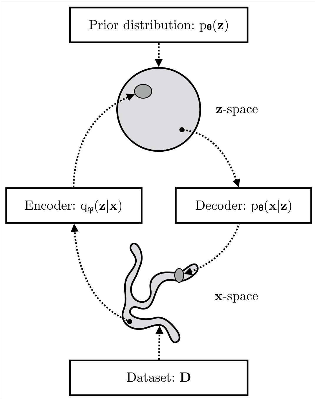
$$ % Define your custom commands here \newcommand{\bmat}[1]{\begin{bmatrix}#1\end{bmatrix}} \newcommand{\E}{\mathbb{E}} \newcommand{\P}{\mathbb{P}} \newcommand{\S}{\mathbb{S}} \newcommand{\R}{\mathbb{R}} \newcommand{\S}{\mathbb{S}} \newcommand{\norm}[2]{\|{#1}\|_{{}_{#2}}} \newcommand{\pd}[2]{\frac{\partial #1}{\partial #2}} \newcommand{\pdd}[2]{\frac{\partial^2 #1}{\partial #2^2}} \newcommand{\vectornorm}[1]{\left|\left|#1\right|\right|} \newcommand{\abs}[1]{\left|{#1}\right|} \newcommand{\mbf}[1]{\mathbf{#1}} \newcommand{\mc}[1]{\mathcal{#1}} \newcommand{\bm}[1]{\boldsymbol{#1}} \newcommand{\nicefrac}[2]{{}^{#1}\!/_{\!#2}} \newcommand{\argmin}{\operatorname*{arg\,min}} \newcommand{\argmax}{\operatorname*{arg\,max}} \newcommand{\dd}{\operatorname{d}\!} $$

Variational Autoencoders

Variational autoencoders (VAEs) are probabilisitic generative models.
- They aim to learn a distribution $p(x)$ over the data.
- After training, it is possible to draw (generate) samples from this distribution.
- Unfortunately, it is not possible to compute the log-likelihood of a sample $x^*$ exactly.
It is possible to define a lower bound on the likelihood.
- The VAE approximates this bound using a Monte Carlo sampling approach.

Image credits: Understanding Deep Learning by Simon J. D. Prince, [CC BY 4.0] and
An Introduction to Variational Autoencoders by Kingma, D. P. and Welling, M.

Credits: Introduction to Flow Matching and Diffusion Models by Peter Holderrieth

Image credits: Understanding Deep Learning by Simon J. D. Prince, [CC BY 4.0]

Linear latent variable models

LVMs model a joint distribution $p(\bm{x}, \bm{z})$ of the data $\bm{x}$ and a latent variable $\bm{z}$.
They then describe $p(\bm{x})$ as the marginal distribution of the joint distribution: \[ p(\bm{x}) = \int p(\bm{x}, \bm{z}) d\bm{z} = \int p(\bm{x} | \bm{z}) p(\bm{z}) d\bm{z}. \]
This is a rather indirect approach to describint $p(\bm{x})$.
- Useful because expressions for $p(\bm{x} | \bm{z})$ and $p(\bm{z})$ are often much simpler than that for $p(\bm{x})$.

Example: Gaussian Mixture Models

Let’s take a $1$D mixture of Gaussians
- $z$ is discrete: $p(z)$ is a categorical distribution with probability $\lambda_n$ for every possible value of $z$.
- The likelihood $p(x \mid z = n)$ of the data is normally distributed with mean $\mu_n$ and variance $\sigma_n^2$. \[ \begin{aligned} p(z = n) &= \lambda_n \\ p(x \mid z = n) &= \mathcal{N}(x \mid \mu_n, \sigma_n^2). \end{aligned} \]
The data likelihood is given by marginalizing over the latent variable $z$ \[ p(x) = \sum_{n=1}^N p(x, z=n) = \sum_{n=1}^N p(x \mid z=n) p(z=n) = \sum_{n=1}^N \lambda_n \mathcal{N}(x \mid \mu_n, \sigma_n^2). \]
Note that the likelihood and prior are both simple expressions, but the resulting data likelihood is multimodal!

Mixture of Gaussians (MoG). a) The MoG describes a complex probability distribution (cyan curve) as a weighted sum of Gaussian components (dashed curves). b) This sum is the marginalization of the joint density p(x, z) between the continuous observed data x and a discrete latent variable z. — Mixture of Gaussians (MoG).
a) The MoG describes a complex probability distribution (cyan curve) as a weighted sum of Gaussian components (dashed curves).
b) This sum is the marginalization of the joint density $p(x, z)$ between the continuous observed data $x$ and a discrete latent variable $z$.

Nonlinear latent variable models

In a nonlinear latent variable model, both the data $\bm{x}$ and the latent variable $\bm{z}$ are continuous and multivariate.

Both the prior $p(\bm{z})$ and the likelihood $p(\bm{x} \mid \bm{z})$ are normally distributed.
- $p(\bm{z}) = \mathcal{N}(\bm{z} \mid \bm{0}, \bm{I})$
- $p(\bm{x} \mid \bm{z}, \bm{\theta}) = \mathcal{N}(\bm{x} \mid \mu(\bm{z}), \Sigma(\bm{z}))$
Say, the likelihood is modeling a continuous variable: the mean and covariance are given by neural networks
- Many times the covariance is fixed and assumed to be diagonal: $\Sigma(\bm{z}) = \sigma^2 \bm{I}$ ($\sigma$ can be learned, too)
- The mean is given by a neural network: $\mu(\bm{z}) = f(\bm{z}; \bm{\theta})$
The latent variable $\bm{z}$ is lower dimensional than the data $\bm{x}$.
In this example, the data probability $p(\bm{x} \mid \bm{\theta})$ is found by marginalizing over the latent variable $\bm{z}$ \[ p(\bm{x} \mid \bm{\theta}) = \int p(\bm{x} \mid \bm{z}, \bm{\theta}) p(\bm{z}) d\bm{z} = \int \mathcal{N}\left(\bm{x} \mid f(\bm{z}; \bm{\theta}), \sigma^2 \bm{I}\right) \mathcal{N}(\bm{z} \mid \bm{0}, \bm{I}) d\bm{z} \]

Nonlinear latent variable model. A complex 2D density p(\bm{x}) (right) is created as the marginalization of the joint distribution p(\bm{x}, z) (left) over the latent variable z; to create p(\bm{x}), we integrate the 3D volume over the dimension z. For each z, the distribution over \bm{x} is a spherical Gaussian (two slices shown) with a mean f(\bm{z}; \bm{\theta}) that is a nonlinear function of z and depends on parameters \theta. The distribution p(\bm{x}) is a weighted sum of these Gaussians. — Nonlinear latent variable model. A complex $2$D density $p(\bm{x})$ (right) is created as the marginalization of the joint distribution $p(\bm{x}, z)$ (left) over the latent variable $z$; to create $p(\bm{x})$, we integrate the $3$D volume over the dimension $z$. For each $z$, the distribution over $\bm{x}$ is a spherical Gaussian (two slices shown) with a mean $f(\bm{z}; \bm{\theta})$ that is a nonlinear function of $z$ and depends on parameters $\theta$. The distribution $p(\bm{x})$ is a weighted sum of these Gaussians.

This can be viewed as an infinite weighted sum (i.e., an infinite mixture)
- Mixture is of spherical Gaussians with different means
- The weights are $p(\bm{z})$ and the means are $f(\bm{z}; \bm{\theta})$

Generation

A new example $\bm{x}^*$ is generated by ancestral sampling.

Draw $\bm{z}^* \sim p(\bm{z})$
Draw $\bm{x}^* \sim p(\bm{x} \mid \bm{z}^*)$
- Pass $\bm{z}^*$ through the decoder network $f(\bm{z}^*; \bm{\theta})$ to compute the mean of $p(\bm{x} \mid \bm{z}^*)$
- Draw $\bm{x}^*$ from $\mathcal{N}(\bm{x}^* \mid f(\bm{z}^*; \bm{\theta}), \sigma^2 \bm{I})$

Generation from nonlinear latent variable model. a) We draw a sample z^* from the prior probability p(z) over the latent variable. b) A sample \bm{x}^* is then drawn from p(\bm{x} \mid z^*, \bm{\theta}). This is a spherical Gaussian with a mean that is a nonlinear function f(\cdot; \bm{\theta}) of z^* and a fixed variance \sigma^2 \bm{I}. c) If we repeat this process many times, we recover the density p(\bm{x} \mid \bm{\theta}). — Generation from nonlinear latent variable model. a) We draw a sample $z^*$ from the prior probability $p(z)$ over the latent variable. b) A sample $\bm{x}^*$ is then drawn from $p(\bm{x} \mid z^*, \bm{\theta})$. This is a spherical Gaussian with a mean that is a nonlinear function $f(\cdot; \bm{\theta})$ of $z^*$ and a fixed variance $\sigma^2 \bm{I}$. c) If we repeat this process many times, we recover the density $p(\bm{x} \mid \bm{\theta})$.

Training

We want to maximize the log-likelihood over a training dataset $\{ \bm{x}_i \}_{i=1}^I$ with respect to $\bm{\theta}$ \[ \bm{\theta}^* = \arg\max_{\bm{\theta}} \sum_{i=1}^I \log p(\bm{x}_i \mid \bm{\theta}) = \argmax_{\bm{\theta}} \sum_{i=1}^I \log \int p(\bm{x}_i \mid \bm{z}, \bm{\theta}) p(\bm{z}) d\bm{z}, \tag{1}\] where for the Gaussian likelihood example, we would have \[ p(\bm{x}_i \mid \bm{\theta}) = \int \mathcal{N}\left(\bm{x}_i \mid f(\bm{z}; \bm{\theta}), \sigma^2 \bm{I}\right) \mathcal{N}(\bm{z} \mid \bm{0}, \bm{I}) d\bm{z}. \]
Unfortunately, this is intractable to compute directly.
- No closed-form expression for the integral
- No easy way to evaluate it for a particular value of $\bm{x}$
To make progress, we define a lower bound on the log-likelihood.
- Always less than or equal to the log-likelihood for a given value of $\bm{\theta}$
- Depends on some other parameters $\bm{\phi}$
- We will build a network to compute this lower bound and optimize it.

Jensen’s inequality

A concave function $g(\cdot)$ of the expectation of data $y$ is greater than or equal to the expectation of the function of the data: \[ g\left(\mathbb{E}[y]\right) \geq \mathbb{E}[g(y)]. \]

Using Jensen’s equality with $g = \log$, we obtain \[ \log \E(y) = \log \int p(y)y dy \geq \int p(y) \log{(y)} dy = \E \log{y}. \]
In fact, the slightly more general statement is true: \[ \log \int p(y)h(y)dy \geq \int p(y) \log{(h(y))}dy, \] for some function $h(y)$ of $y$.
The intractability of $p(\bm{x} \mid \theta)$ is related to the intractability of the posterior distribution $p(\bm{z} \mid \bm{x}, \bm{\theta})$.
- Note that the joint distribution $p(\bm{x}, \bm{z} \mid \theta)$ is efficient to compute and we have \[ p(\bm{z} \mid \bm{x}, \bm{\theta}) = \frac{p(\bm{x}, \bm{z} \mid \bm{\theta})}{p(\bm{x} \mid \bm{\theta})} \]
- Since $p(\bm{x}, \bm{z} \mid \bm{\theta})$ is tractable to compute, a tractable marginal likelihood $p(\bm{x} \mid \bm{\theta})$ leads to a tractable posterior $p(\bm{z} \mid \bm{x}, \bm{\theta})$, and vice versa. Both are intractable!

Posterior distribution over the latent variable. a) The posterior distribution p(z \mid \bm{x}^*, \bm{\theta}) is the distribution over the values of the latent variable z that could be responsible for a data point \bm{x}^*. We calculate this via Bayes’s rule p(z \mid \bm{x}^*, \bm{\theta}) \propto p(\bm{x}^* \mid z, \bm{\theta}) p(z). b) We compute the first term on the right hand side (the likelihood) by assessing the probability of \bm{x}^* against the symmetric Gaussian associated with each value of z. Here, it was more likely to have been created from z_1 than z_2. The second term is the prior probability p(z) over the latent variable. Combining these two factors and normalizing so the distribution sums to one gives us the posterior distribution p(z \mid \bm{x}^*, \bm{\theta}). — Posterior distribution over the latent variable. a) The posterior distribution $p(z \mid \bm{x}^*, \bm{\theta})$ is the distribution over the values of the latent variable $z$ that could be responsible for a data point $\bm{x}^*$. We calculate this via Bayes’s rule $p(z \mid \bm{x}^*, \bm{\theta}) \propto p(\bm{x}^* \mid z, \bm{\theta}) p(z)$. b) We compute the first term on the right hand side (the likelihood) by assessing the probability of $\bm{x}^*$ against the symmetric Gaussian associated with each value of $z$. Here, it was more likely to have been created from $z_1$ than $z_2$. The second term is the prior probability $p(z)$ over the latent variable. Combining these two factors and normalizing so the distribution sums to one gives us the posterior distribution $p(z \mid \bm{x}^*, \bm{\theta})$.

Let us introduce a parametric inference model $q(\bm{z} \mid \bm{x}, \bm{\phi})$.
- Also called an encoder or recognition model.
- With $\bm{\phi}$, we indicate the variational parameters.
- We optimize the variational parameters $\bm{\phi}$ such that \[ q(\bm{z} \mid \bm{x}, \bm{\phi}) \approx p(\bm{z} \mid \bm{x}, \bm{\theta}). \]
For any choice of inference model $q(\bm{z} \mid \bm{x}, \bm{\phi})$, including the choice of variational parameters $\bm{\phi}$, we have \[ \begin{aligned} \log p(\bm{x} \mid \bm{\theta}) &= \E_{q(\bm{z} \mid \bm{x}, \bm{\phi})}[\log p(\bm{x} \mid \bm{\theta})] \\ &= \E_{q(\bm{z} \mid \bm{x}, \bm{\phi})}\left[ \log \left( \frac{p(\bm{x}, \bm{z} \mid \bm{\theta})}{p(\bm{z} \mid \bm{x}, \bm{\theta})} \right) \right] \\ &= \E_{q(\bm{z} \mid \bm{x}, \bm{\phi})}\left[ \log \left( \frac{p(\bm{x}, \bm{z} \mid \bm{\theta})}{q(\bm{z} \mid \bm{x}, \bm{\phi})} \frac{q(\bm{z} \mid \bm{x}, \bm{\phi})}{p(\bm{z} \mid \bm{x}, \bm{\theta})} \right) \right] \\ &= \underbrace{\E_{q(\bm{z} \mid \bm{x}, \bm{\phi})}\left[ \log \left( \frac{p(\bm{x}, \bm{z} \mid \bm{\theta})}{q(\bm{z} \mid \bm{x}, \bm{\phi})} \right) \right]}_{=\mc{L}_{\theta, \phi}(x) \\[1pt] \text{(ELBO)}} + \underbrace{\E_{q(\bm{z} \mid \bm{x}, \bm{\phi})}\left[ \log \left( \frac{q(\bm{z} \mid \bm{x}, \bm{\phi})}{p(\bm{z} \mid \bm{x}, \bm{\theta})} \right) \right]}_{=D_{\text{KL}}(q(\bm{z} \mid \bm{x}, \bm{\phi})\;\Vert\; p(\bm{z} \mid \bm{x}, \bm{\theta}))} \end{aligned} \tag{2}\]
The second term is the Kullback-Leibler (KL) divergence which is nonnegative: \[ D_{\text{KL}}(q(\bm{z} \mid \bm{x}, \bm{\phi})\;\Vert\; p(\bm{z} \mid \bm{x}, \bm{\theta})) \geq 0 \] and zero if and only if $q(\bm{z} \mid \bm{x}, \bm{\phi}) = p(\bm{z} \mid \bm{x}, \bm{\theta})$.
The first term is the variational lower bound, also called the evidence lower bound (ELBO): \[ \mc{L}_{\theta, \phi}(x) = \E_{q_\phi(\bm{z} \mid \bm{x})} \left[ \log p_\theta(\bm{x}, \bm{z}) - \log q_\phi(\bm{z} \mid \bm{x}) \right] \tag{3}\]
Due to the nonnegativity of the KL divergence, the ELBO is a lower bound on the log-likelihood of the data: \[ \mc{L}_{\theta, \phi}(\bm{x}) = \log p_\theta(\bm{x}) - D_{\text{KL}}\left(q_\phi(\bm{z} \mid \bm{x})\,\Vert\,p_\theta(\bm{z} \mid \bm{x})\right) \leq \log p_\theta(\bm{x}). \tag{4}\]
Hence, the KL divergence $D_{\text{KL}}\left(q_\phi(\bm{z} \mid \bm{x})\,\Vert\,p_\theta(\bm{z} \mid \bm{x})\right)$ determines two “distances”:
1. By definition, the KL divergence of the approximate posterior from the true posterior.
2. The gap between the ELBO $\mc{L}_{\theta, \phi}(\bm{x})$ and the marginal likelihood $\log p_\theta(\bm{x})$.
- The latter is also called the tightness of the bound.
- The better $q_\phi(\bm{z} \mid \bm{x})$ approximates the true (posterior) distribution $p_\theta(\bm{z} \mid \bm{x})$, in terms of the KL divergence, the smaller the gap.

$Variational approximation. The posterior p(\bm{z} \mid \bm{x}^*, \bm{\theta}) is intractable to compute. The variational approximation chooses a family of distributions q(\bm{z} \mid \bm{x}, \bm{\phi}) (here Gaussians) and tries to find the closest member of this family to the true posterior. a) Sometimes, the approximation (cyan curve) is good and lies close tot he true posterior (orange curve). b) However, if the posterior is multi-modal (as in the previous figure), then the Gaussian approximation will be poor.$

Variational approximation. The posterior $p(\bm{z} \mid \bm{x}^*, \bm{\theta})$ is intractable to compute. The variational approximation chooses a family of distributions $q(\bm{z} \mid \bm{x}, \bm{\phi})$ (here Gaussians) and tries to find the closest member of this family to the true posterior. a) Sometimes, the approximation (cyan curve) is good and lies close tot he true posterior (orange curve). b) However, if the posterior is multi-modal (as in the previous figure), then the Gaussian approximation will be poor.

Two for One

By looking at Equation 4, it can be understood that maximization of the ELBO $\mc{L}_{\theta, \phi}(x)$ with respect to $\bm{\theta}$ and $\bm{\phi}$, will concurrently optimize the two things we care about:

It will approximately maximize the marginal likelihood $p_\theta(\bm{x})$. This means that our generative model or decoder will become better.
It will minimize the KL divergence of the approximation $q_\phi(\bm{z} \mid \bm{x})$ from the true posterior $p_\theta(\bm{z} \mid \bm{x})$, so $q_\phi(\bm{z} \mid \bm{x})$ becomes better.

ELBO through Jensen’s inequality

We can also see that the ELBO is a lower bound on the log-likelihood by using Jensen’s inequality. \[ \begin{aligned} \log p(\bm{x} \mid \bm{\theta}) &= \log \int p(\bm{x}, \bm{z} \mid \bm{\theta}) d\bm{z} = \log \int p(\bm{x}, \bm{z} \mid \bm{\theta}) \frac{q(\bm{z} \mid \bm{x}, \bm{\phi})}{q(\bm{z} \mid \bm{x}, \bm{\phi})} d\bm{z} = \log \E_{q(\bm{z} \mid \bm{x}, \bm{\phi})} \left[ \frac{p(\bm{x}, \bm{z} \mid \bm{\theta})}{q(\bm{z} \mid \bm{x}, \bm{\phi})} \right] \\ &\geq \E_{q(\bm{z} \mid \bm{x}, \bm{\phi})} \left[ \log \frac{p(\bm{x}, \bm{z} \mid \bm{\theta})}{q(\bm{z} \mid \bm{x}, \bm{\phi})} \right] = \mc{L}_{\theta, \phi}(x) \end{aligned} \]

Evidence lower bound (ELBO). The goal is to maximize the log-likelihood \log p_\theta(\bm{x}) (black curve) with respect to the parameters \bm{\theta}. The ELBO is a function that lies everywhere below the log-likelihood. It is a function of both \bm{\theta} and a second set of parameters \bm{\phi}. For fixed \bm{\phi}, we get a function of \bm{\theta} (two colored curves for different values of \bm{\phi}). Consequently, we can increase the log-likelihood by either improving the ELBO with respect to a) the new parameters \bm{\phi} (moving from colored curve to colored curve) or b) the original parameters \bm{\theta} (moving along the current colored curve). — Evidence lower bound (ELBO). The goal is to maximize the log-likelihood $\log p_\theta(\bm{x})$ (black curve) with respect to the parameters $\bm{\theta}$. The ELBO is a function that lies everywhere below the log-likelihood. It is a function of both $\bm{\theta}$ and a second set of parameters $\bm{\phi}$. For fixed $\bm{\phi}$, we get a function of $\bm{\theta}$ (two colored curves for different values of $\bm{\phi}$). Consequently, we can increase the log-likelihood by either improving the ELBO with respect to a) the new parameters $\bm{\phi}$ (moving from colored curve to colored curve) or b) the original parameters $\bm{\theta}$ (moving along the current colored curve).

Two Models to Learn

Encoder or Recognition or Inference Model \[ \begin{aligned} (\bm{\mu}, \log \bm{\sigma}) &= \operatorname{EncoderNeuralNet}_\phi(\bm{x}) \\ q_\phi(\bm{z} \mid \bm{x}) &= \mc{N}(\bm{z}; \bm{\mu}, \operatorname{diag}{(\bm{\sigma})}). \end{aligned} \]
Decoder or Generative Model (Binary Data) \[ \begin{aligned} \bm{p} &= \operatorname{DecoderNeuralNet_\theta(\bm{z})} \\ \log p_\theta(\bm{x} \mid \bm{z}) &= \sum_{j=1}^D \log p(x_j \mid \bm{z}) = \sum_{j=1}^D \operatorname{Bernoulli(x_j; p_j)} \\ &= \sum_{j=1}^D \left[ x_j \log p_j + (1-x_j) \log(1-p_j) \right] \end{aligned} \] where $\forall p_j \in \bm{p}; 0 \leq p_j \leq 1$ (e.g. implemented through a sigmoid nonlinearity as the last layer of the $\operatorname{DecoderNeuralNet}_\theta(\cdot)$), where $D$ is the dimensionality of $\bm{x}$, and $\operatorname{Bernoulli}(\cdot; p)$ is the probability mass function of the Bernoulli distribution.

Summary

Since we the log-likelihood is intractable to compute, we cannot perform the optimization in Equation 1. Instead, we will maximize the ELBO $\mc{L}_{\theta, \phi}(x)$ with respect to both the decoder and encoder $(\bm{\theta}, \bm{\phi})$ as a proxy.

Variational autoencoder. The encoder g(\bm{x}; \bm{\theta}) takes a training example \bm{x} and predicts the parameters \bm{\mu}, \bm{\Sigma} of the variational distribution q_\theta(\bm{z} \mid \bm{x}). We sample from this distribution and then use the decoder f(\bm{z}; \bm{\phi}) to predict the data \bm{x}. The loss function is the negative ELBO, which depends on how accurate this prediction is and how similar the variational distribution q_\phi(\bm{z} \mid \bm{x}) is to the prior p(\bm{z}). — Variational autoencoder. The encoder $g(\bm{x}; \bm{\theta})$ takes a training example $\bm{x}$ and predicts the parameters $\bm{\mu}, \bm{\Sigma}$ of the variational distribution $q_\theta(\bm{z} \mid \bm{x})$. We sample from this distribution and then use the decoder $f(\bm{z}; \bm{\phi})$ to predict the data $\bm{x}$. The loss function is the negative ELBO, which depends on how accurate this prediction is and how similar the variational distribution $q_\phi(\bm{z} \mid \bm{x})$ is to the prior $p(\bm{z})$.

How to maximize ELBO?

Unbiased gradients of the ELBO with respect to the generative model parameters $\bm{\theta}$ are simple to obtain: \[ \begin{aligned} \nabla_\theta \mc{L}_{\theta, \phi}(x) &= \nabla_\theta \E_{q_\phi(\bm{z} \mid \bm{x})} \left[\log p_\theta(\bm{x}, \bm{z}) - \log q_\phi(\bm{z} \mid \bm{x}) \right] \\ &= \E_{q_\phi(\bm{z} \mid \bm{x})} \left[\nabla_\theta\left( \log p_\theta(\bm{x}, \bm{z}) - \log q_\phi(\bm{z} \mid \bm{x}) \right) \right] \\ &\simeq \nabla_\theta\left( \log p_\theta(\bm{x}, \bm{z}) - \log q_\phi(\bm{z} \mid \bm{x}) \right) \\ &= \nabla_\theta \log p_\theta(\bm{x}, \bm{z}). \end{aligned} \] The last line is a simple Monte Carlo estimator of the second line, where $\bm{z}$ in the last two lines is a random sample from $q_\phi(\bm{z} \mid \bm{x})$.
Unbiased gradients with respect to the variational parmaeters $\bm{\phi}$ are more difficult to obtain.
- ELBO’s expectation is taken with respect to the distribution $q_\phi(\bm{z} \mid \bm{x})$.
- This is a function of $\bm{\phi}$!

\[ \begin{aligned} \nabla_\phi \mc{L}_{\theta, \phi}(\bm{x}) &= \nabla_\phi \E_{q_\phi(\bm{z} \mid \bm{x})} \left[\log p_\theta(\bm{x}, \bm{z}) - \log q_\phi(\bm{z} \mid \bm{x}) \right] \\ &\neq \E_{q_\phi(\bm{z} \mid \bm{x})} \left[\nabla_\phi \left( \log p_\theta(\bm{x}, \bm{z}) - \log q_\phi(\bm{z} \mid \bm{x}) \right) \right] \end{aligned} \]

The reparametrization trick (law of the unconscious statistician: lotus)

For continuous latent variables and a differentiable encoder and generative model, the ELBO can be straightforwardly differentiated with respect to both $\bm{\phi}$ and $\bm{\theta}$ through a change of variables, also called the reparametrization trick.

Express the random variable $\bm{z} \sim q_\phi(\bm{z} \mid \bm{x})$ as some differentiable (and invertible) transformation.
- This is a function of another random variable $\bm{\varepsilon}$, given $\bm{z}$ and $\bm{\phi}$: \[ \bm{z} = \bm{h}(\bm{\varepsilon}, \bm{\phi}, \bm{x}) \]
- The random variable $\bm{\varepsilon}$ is independent of $\bm{x}$ or $\bm{\phi}$.
Now, the expectations can be rewritten in terms of $\bm{\varepsilon}$: \[ \E_{q_\phi(\bm{z} \mid \bm{x})}[f(\bm{z})] = \E_{p(\bm{\varepsilon})}[f(\bm{z})]. \]
This makes the expectation and gradient operators commutative, and we can form a simple Monte Carlo estimator: \[ \begin{aligned} \nabla_\phi \E_{q_\phi(\bm{z} \mid \bm{x})}[f(\bm{z})] &= \nabla_\phi \E_{p(\bm{\varepsilon})}[f(\bm{z})] \\ &= \E_{p(\bm{\varepsilon})}[\nabla_\phi f(\bm{z})] \\ &\simeq \nabla_\phi f(\bm{z}) \end{aligned} \] where in the last line, $\bm{z} = h(\bm{\varepsilon}, \bm{\phi}, \bm{x})$ with random noise sample $\bm{\varepsilon} \sim p(\bm{\varepsilon})$.

Reparametrization trick. The variational parameters \bm{\phi} affect the objective f through the random variable \bm{z} \sim q_\phi(\bm{z} \mid \bm{x}). We wish to compute gradients \nabla_\phi f to optimize the objective with SGD. In the original form (left), we cannot differentiate f w.r.t. \bm{\phi}, because we cannot directly backpropagate gradients through the random variable \bm{z}. We can “externalize” the randomness in \bm{z} by re-parametrizing the variable as a deterministic and differentiable function of \bm{\phi}, bm{x}, and a newly introduced random variable \bm{\varepsilon} (right). This allows us to “backprop through \bm{z},” and compute gradients \nabla_\phi f. — Reparametrization trick. The variational parameters $\bm{\phi}$ affect the objective $f$ through the random variable $\bm{z} \sim q_\phi(\bm{z} \mid \bm{x})$. We wish to compute gradients $\nabla_\phi f$ to optimize the objective with SGD. In the original form (left), we cannot differentiate $f$ w.r.t. $\bm{\phi}$, because we cannot directly backpropagate gradients through the random variable $\bm{z}$. We can “externalize” the randomness in $\bm{z}$ by re-parametrizing the variable as a deterministic and differentiable function of $\bm{\phi}$, $bm{x}$, and a newly introduced random variable $\bm{\varepsilon}$ (right). This allows us to “backprop through $\bm{z}$,” and compute gradients $\nabla_\phi f$.

Gradient of ELBO

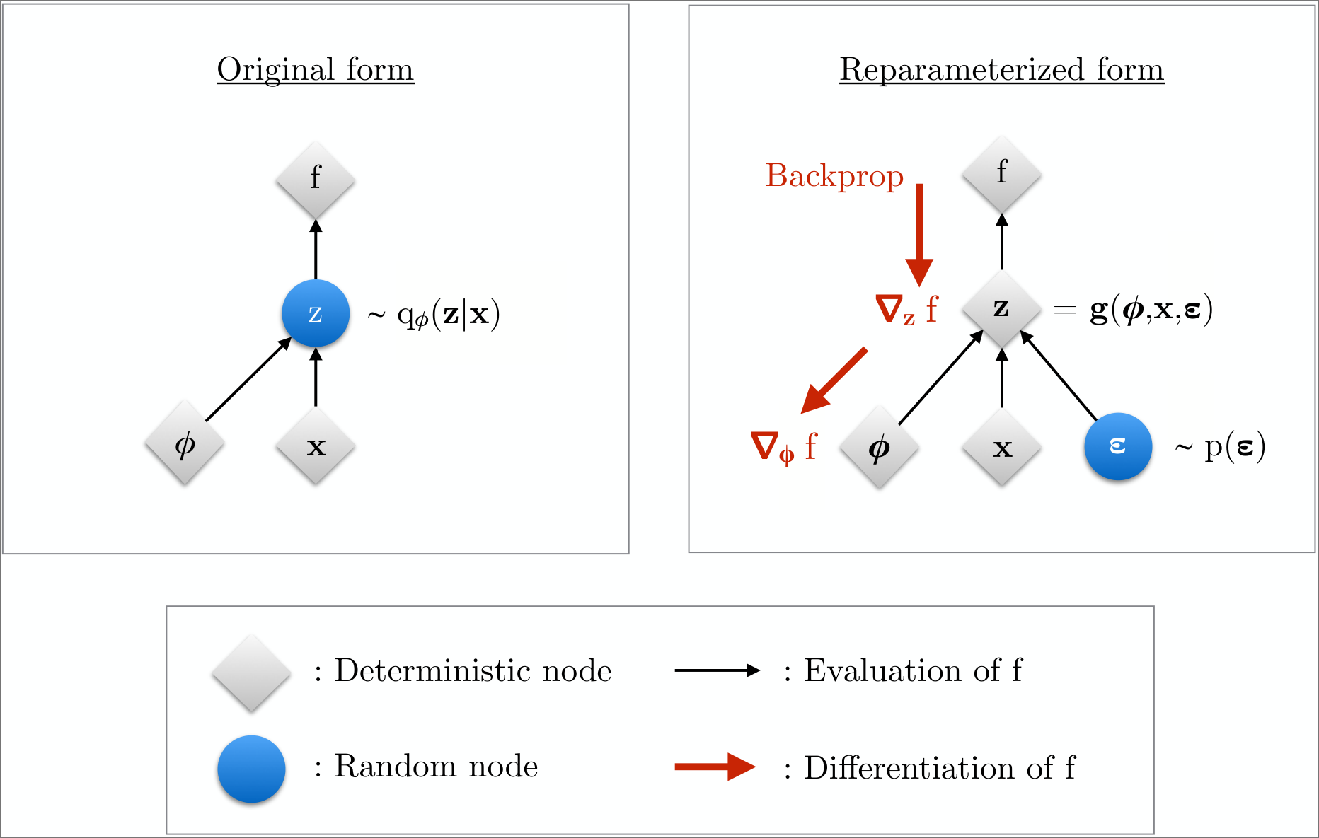
Under the reparametrization, we can replace an expectation with respect to $q_\phi(\bm{z} \mid \bm{x})$ with one with respect to $p(\bm{\varepsilon})$.
- Now, the ELBO can be written as \[ \begin{aligned} \mc{L}_{\theta, \phi}(\bm{x}) &= \E_{q_\phi(\bm{z} \mid \bm{x})} \left[ \log p_\theta(\bm{x}, \bm{z}) - \log q_\phi(\bm{z} \mid \bm{x}) \right] \\ &= \E_{p(\bm{\varepsilon})} \left[ \log p_\theta(\bm{x}, \bm{z}) - \log q_\phi(\bm{z} \mid \bm{x}) \right], \end{aligned} \] where $\bm{z} = \bm{h}(\bm{\varepsilon}, \bm{\phi}, \bm{x})$.
As a result, we can form a simple Monte Carlo estimator $\tilde{\mc{L}}_{\theta, \phi}(\bm{x})$: \[ \begin{aligned} \bm{\varepsilon} &\sim p(\bm{\varepsilon}) \\ \bm{z} &= \bm{h}(\bm{\varepsilon}, \bm{\phi}, \bm{x}) \\ \tilde{\mc{L}}_{\theta, \phi}(\bm{x}) &= \log p_\theta(\bm{x}, \bm{z}) - \log q_\phi(\bm{z} \mid \bm{x}) \end{aligned} \]
The resulting gradient $\nabla_\phi \tilde{\mc{L}}_{\theta, \phi}(\bm{x})$ is used to optimize the ELBO using minibatch SGD.

Reparametrization trick. With the original architecture, we cannot easily backpropagate through the sampling step. The reparametrization trick removes the sampling step from the main pipeline; we draw from a standard normal and combine this with the predicted mean and covariance to get a sample from the variational distribution.

The VAE updates both factors that determine the lower bound at each iteration. Both parameters \bm{\theta} of the decoder and the parameters \bm{\theta} of the encoder are manipulated to increase this lower bound. — The VAE updates both factors that determine the lower bound at each iteration. Both parameters $\bm{\theta}$ of the decoder and the parameters $\bm{\theta}$ of the encoder are manipulated to increase this lower bound.

Both the encoder and the decoder give rise to a joint distribution over both $x$ and the latent $z$, that is, \[ \begin{aligned} q_\phi(x, z) &= p_{\text{data}}(x) q_\phi(z \mid x) \\ p_\theta(x, z) &= p_\theta(x \mid z) p_{\text{prior}}(z) \end{aligned} \]
Conceptualize training the VAE as learning $\phi$ and $\theta$ so that the encoder and decoder joint distributions are reasonably similar.
- Do this via minimizing the KL-divergence of the joint latent and data distributions: \[ \begin{aligned} D_{\text{KL}}\left(q_\phi(x, z)\, \|\, p_\theta(x, z)\right) &= D_{\text{KL}}\left( p_{\text{data}}(x) q_\phi(z \mid x)\, \|\, p_\theta(x \mid z) p_{\text{prior}}(z) \right) \\ &= \E_\blacksquare \left[ \log \left( \frac{p_{\text{data}}(x) q_\phi(z \mid x)}{p_\theta(x \mid z) p_{\text{prior}}(z)} \right) \right] \\ &= \textcolor{#1f77b4}{\E_\blacksquare\left[\log p_{\text{data}}(x)\right]} + \textcolor{#ff7f0e}{\E_\blacksquare\left[\log \frac{q_\phi(z \mid x)}{p_{\text{prior}}(z)}\right]} - \textcolor{#2ca02c}{\E_\blacksquare\left[\log p_\theta(x \mid z)\right]} \\ \blacksquare &= x \sim p_{\text{data}}(x), \, z \sim q_\phi(z \mid x) \end{aligned} \]
Analyze the first term: \[ \textcolor{#1f77b4}{\E_\blacksquare\left[\log p_{\text{data}}(x)\right] = \E_{x \sim p_{\text{data}}(x)}[\log p_{\text{data}}(x)] = C, } \] for some constant $C$ independent of $\phi$ and $\theta$.
Analyze the second term: \[ \textcolor{#ff7f0e}{\E_\blacksquare\left[\log \frac{q_\phi(z \mid x)}{p_{\text{prior}}(z)}\right] = \E_{x \sim p_{\text{data}}(x)} \left[ D_{\text{KL}}(q_\phi(z \mid x)\, \|\, p_{\text{prior}}(z)) \right] } \] encourages $q_\phi(z \mid x)$ to resemble the prior $p_{\text{prior}}(z)$.
Analyze the third term: \[ -\textcolor{#2ca02c}{\E_\blacksquare\left[\log p_\theta(x \mid z)\right] = -\E_{x \sim p_{\text{data}}(x), z \sim q_\phi(z \mid x)}[\log p_\theta(x \mid z)] } \] corresponds to the average negative log-likelihood, and thus serves to minimize the reconstruction loss.
Ignoring the constant term, we combine the and terms to obtain that the VAE loss is actually simply the KL-divergence in joint data and latent space: \[ \begin{aligned} \mc{L}_{\text{VAE}}(\theta, \phi) &= \underbrace{\textcolor{#ff7f0e}{\E_{x \sim p_{\text{data}}(x)} \left[ D_{\text{KL}}(q_\phi(z \mid x)\, \|\, p_{\text{prior}}(z)) \right]}}_{\text{prior enforcement loss}} - \underbrace{\textcolor{#2ca02c}{\E_{x \sim p_{\text{data}}(x), z \sim q_\phi(z \mid x)}[\log p_\theta(x \mid z)]}}_{\text{reconstruction loss}} \\ &= D_{\text{KL}}\left(q_\phi(x, z)\, \|\, p_\theta(x, z)\right) + \text{const} \end{aligned} \] Therefore, we can interpret the VAE as a KL-divergence in the joint space of latents and images.

VAEs as generative models

Another interpretation of VAEs is as a generative model.

We can generate a sample by setting $z \sim p_{\text{prior}}(z) = \mathcal{N}(0, I)$ and sampling $x \sim p_\theta(\cdot \mid z)$ from the decoder.
The distribution that we would get is given by \[ p_\theta(x) = \int p_\theta(x \mid z) p_{\text{prior}}(z) dz. \]

Proposition 1 (Chain rule) Let $q(x, z)$, $p(x, z)$ be distributions over two variables $x \in \R^{l_1}$, $\R^{l_2}$. Then, it holds that \[ D_{\text{KL}}(q(x, z)\, \|\, p(x, z)) = \E_{x \sim q(x)} \left[ D_{\text{KL}}(q(z \mid x)\, \|\, p(z \mid x)) \right] + D_{\text{KL}}(q(x)\, \|\, p(x)). \] In particular, as the second summand is nonnegative, we obtain the data-processing inequality \[ D_{\text{KL}}(q(x)\, \| \, p(x)) \le D_{\text{KL}}(q(x, z)\, \|\, p(x, z)). \]

Proof. \[ \begin{aligned} D_{\text{KL}}\left(q(x, z) \,\|\, p(x, z)\right) &= \E_{(x, z) \sim q(x, z)} \left[ \log \frac{q(x, z)}{p(x, z)} \right] \\ &= \E_{(x, z) \sim q(x, z)} \left[ \log \frac{q(x) q(z \mid x)}{p(x) p(z \mid x)} \right] \\ &= \E_{x \sim q(x)} \left[ \log \frac{q(x)}{p(x)}\right] + \E_{(x, z) \sim q(x, z)} \left[ \log \frac{q(z \mid x)}{p(z \mid x)} \right] \\ &= D_{\text{KL}}(q(x) \,\|\, p(x)) + \E_{x \sim q(x)} \left[ D_{\text{KL}}(q(z \mid x) \,\|\, p(z \mid x)) \right] \end{aligned} \] where we have repeatedly applied the definition of KL-divergence. $\square$

By Proposition 1, we can now show that \[ \mc{L}_{\text{VAE}}(\phi, \theta) = D_{\text{KL}}\left( q_\phi(x, z) \,\|\, p_\theta(x, z) \right) + \text{const} \ge D_{\text{KL}}(p_{\text{data}}(x) \,\|\, p_\theta(x)) + \text{const}. \tag{5}\] where we used the fact that the $x$-marginal of $q_\phi(x, z)$ is $p_{\text{data}}(x)$.

In other words, the VAE loss inimizes an upper bound on the KL-divergence between the data distribution $p_{\text{data}}$ and the distribution $p_\theta(x)$ generated by the VAE.
- Hence, we can look at VAEs as generative models in their own right.
In the same way, we can show that \[ \mc{L}_{\text{VAE}}(\phi, \theta) = D_{\text{KL}}\left( q_\phi(x, z) \,\|\, p_\theta(x, z) \right) + \text{const} \ge D_{\text{KL}}(q_\phi(z) \,\|\, p_{\text{prior}}(z)) + \text{const}. \tag{6}\] In other words, the VAE objective minimize an upper bound on the KL-divergence between the latent distribution and the prior.

Why not stop at VAEs?

VAEs can be realized as generative models in their own right
- Encoder facilitates the training of a complementary decoder.
- Decoder transforms a Gaussian into the desired distribution
- Samples can be obtained by sampling $z \sim p_{\text{prior}}(z)$ and then $x \sim p_\theta(\cdot \mid z)$.
Why then do we need other models, such as diffusion models?
The answer has to do with the so-called amortization gap between the left and right-hand sides of both Equation 5 and Equation 6.
- This gap is zero if and only if $q_\phi(z \mid x) = p_\theta(z \mid x)$, in which case the encoder represents the true posterior.
- While $D_{\text{KL}}(q_\phi(x, z) \,\|\, p_\theta(x, z))$ is minimized implies $D_{\text{KL}}(q_\phi(z) \,\|\, p_{\text{prior}}(z))$ is minimized (see Equation 6), a decrease in the former does not necessarily imply an equal decrease in the latter.
- Consequently, at the end of training, it is simultaneously true that both $D_{\text{KL}}(q_\phi(x, z) \,\|\, p_\theta(x, z))$ and the amortization gap \[ D_{\text{KL}}(q_\phi(x, z) \,\|\, p_\theta(x, z)) - D_{\text{KL}}(q_\phi(z) \,\|\, p_{\text{prior}}(z)) \] are not completely minimized, so that $q_\phi(z) \ne p_{\text{prior}}(z)$ and $p_\theta(x) \ne p_{\text{data}}(x)$.
Finally, observe that during training, the decoder learns to reconstruct from $q_\phi(z)$ rather than $p_{\text{prior}}(z)$.
- Hence, switching to reconstruction from $p_{\text{prior}}(z)$ during inference would amount to going out of distribution from training.
- In practice, however, this is a feature, rather than a bug.
  - Practice has shown flow and diffusion models to be more capable models, in general, than the convolutional stacks used to implement the VAE decoder.