$$ % Define your custom commands here \newcommand{\bmat}[1]{\begin{bmatrix}#1\end{bmatrix}} \newcommand{\E}{\mathbb{E}} \newcommand{\P}{\mathbb{P}} \newcommand{\S}{\mathbb{S}} \newcommand{\R}{\mathbb{R}} \newcommand{\S}{\mathbb{S}} \newcommand{\norm}[2]{\|{#1}\|_{{}_{#2}}} \newcommand{\pd}[2]{\frac{\partial #1}{\partial #2}} \newcommand{\pdd}[2]{\frac{\partial^2 #1}{\partial #2^2}} \newcommand{\vectornorm}[1]{\left|\left|#1\right|\right|} \newcommand{\abs}[1]{\left|{#1}\right|} \newcommand{\mbf}[1]{\mathbf{#1}} \newcommand{\mc}[1]{\mathcal{#1}} \newcommand{\bm}[1]{\boldsymbol{#1}} \newcommand{\nicefrac}[2]{{}^{#1}\!/_{\!#2}} \newcommand{\argmin}{\operatorname*{arg\,min}} \newcommand{\argmax}{\operatorname*{arg\,max}} \newcommand{\dd}{\operatorname{d}\!} $$

Latest figures

Every figure the wdm package draws for the real record, regenerated with the data.

Every figure wdm plots draws for the current diet, from the real record as of November 18, 2026, regenerated with the presentation’s numbers whenever new days are logged; nothing here is drawn by hand. Each caption says how to read its figure. Click or tap a figure to open it full screen and zoom in.

Weight and body composition
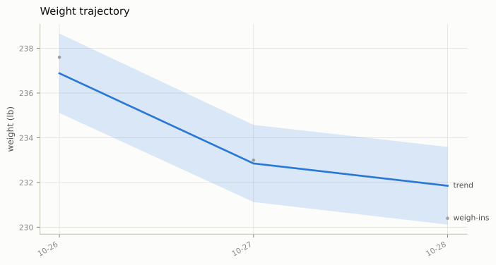
Weight trajectory. Raw weigh-ins (gray), the smoothed trend, and its 95% band. The trend is what moved; the scatter of a pound or more around it is mostly water and gut contents. Judge progress by the trend’s slope over a week or more, never by one morning.

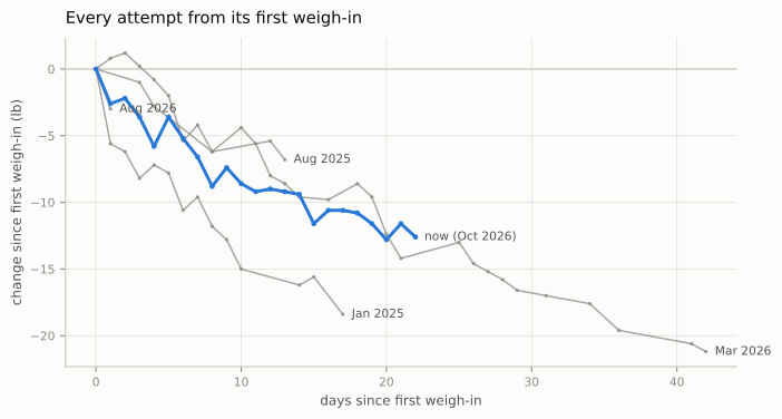
Every attempt. Each diet attempt’s weigh-ins as change since its first weigh-in, against days since it, so attempts that began at different weights and dates line up. The current one is in color; earlier ones are gray, labeled with the month each began. Raw readings joined day to day, not trends; the earlier attempts were weighed less often, so their lines can span days without a reading.

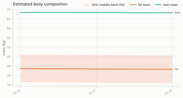
Body composition. Estimated fat and lean mass with their 95% bands. Fat mass enters the dynamics only through the energy density of the tissue lost, so a scale identifies it weakly: read the bands, and the trend rather than the level. Weekly waist readings narrow the fat band somewhat.

The plan

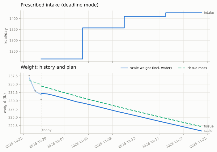
Today’s plan. Top: prescribed intake by week, stacked as protein, carbohydrate and fat. Bottom: predicted scale weight and tissue mass, continuing the filtered trend up to today (faded). The gap between the two lines is water. Only the first day is a prescription; tomorrow the plan is remade and the rest changes.

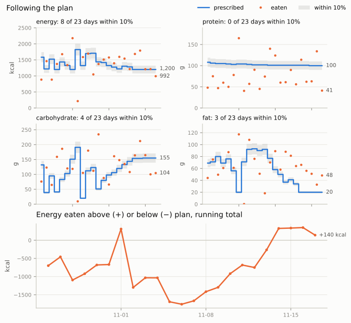
Adherence. Top: energy and each macronutrient eaten on each finished day (dots) against the prescription from the plans log (line), with the range within 10% of it shaded; titles count the days inside that range, and the latest values are labeled. Energy is on the label scale wdm log shows, before the model’s fiber correction. Bottom: the running total of energy eaten above or below plan. That is the panel to watch: a line climbing steadily means the weight will come off more slowly than planned. A macronutrient off on a day when energy is on plan matters less: low protein risks lean mass over weeks, and carbohydrate moves water from day to day, but neither changes how much is lost.

What the model has learned

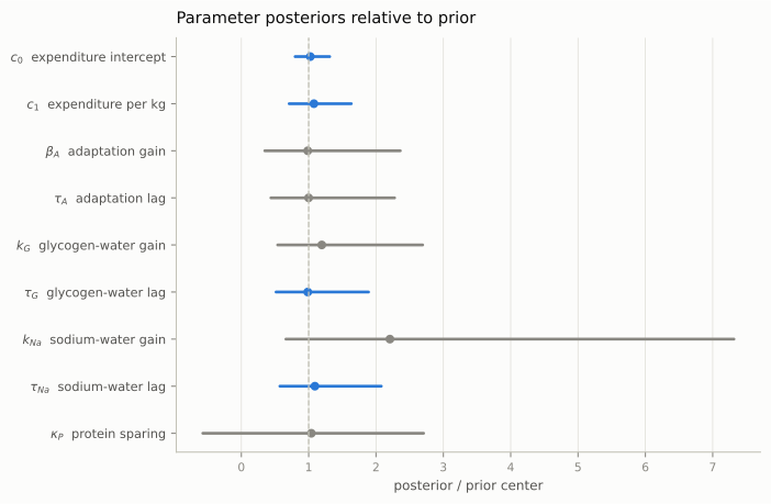
Parameter posteriors. Where each parameter stands today: the posterior median and 90% interval, relative to the prior center (dashed line at 1), drawn over the prior’s own 90% interval (pale bar). The nine metabolic parameters come first, then the waist offset and slope that turn fat mass into waist circumference. A parameter has learned something only where its interval is visibly shorter than the pale bar or sits off-center in it.

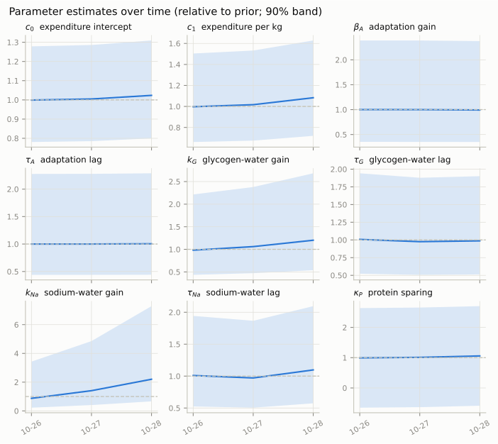
Parameter evolution. What the filter believed about each of the nine metabolic parameters and the two waist parameters, day by day, relative to its prior center (dashed line at 1), with a 90% band. Each day uses only the record up to that morning. Read the band’s width: a band as wide as it started has learned nothing, whatever its median does. A band that has narrowed and moved off the line is where the data have spoken.

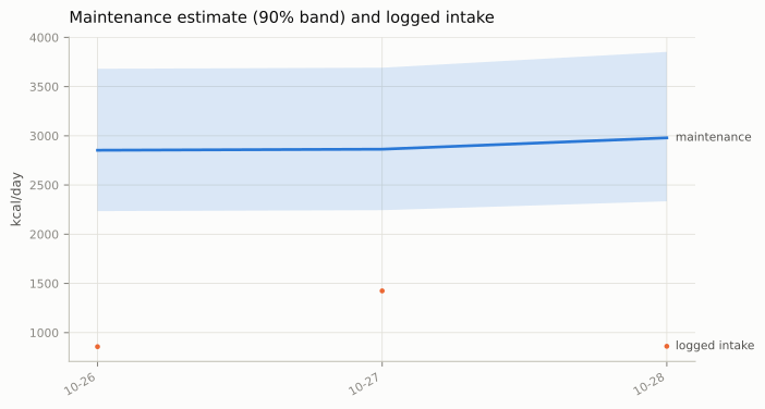
Maintenance. Energy spent at each day’s tissue mass, \(c_0 + c_1 T\) (water and gut content cost nothing to maintain), as the filter estimated it (90% band), against the logged intake on the same axis; the vertical gap between them is the day’s deficit. The band is narrow even when the two coefficients behind it are not, because their errors are strongly correlated (why).

Diagnostics and inputs

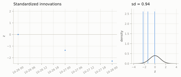
Innovations. Each weigh-in’s one-step-ahead surprise, in standard deviations, over time and as a histogram. An adequate model’s are centered on zero with a standard deviation near 1 and no pattern. A histogram wider than the reference curve means the noise is understated and the intervals overconfident; a weekly pattern usually means weekend eating the log misses (Troubleshooting).

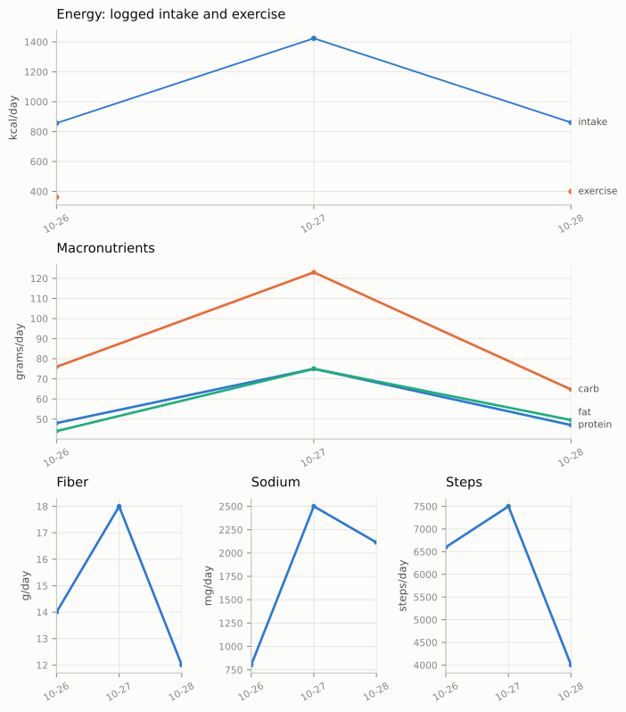
Intake log. Exercise energy, fiber, sodium, and steps logged in the current diet. Unlogged days are left blank, so that a missing reading is never drawn as a measured one.