An energy-balance state-space model, a joint unscented Kalman filter, and a receding-horizon diet controller
Aykut C. Satici
November 16, 2026
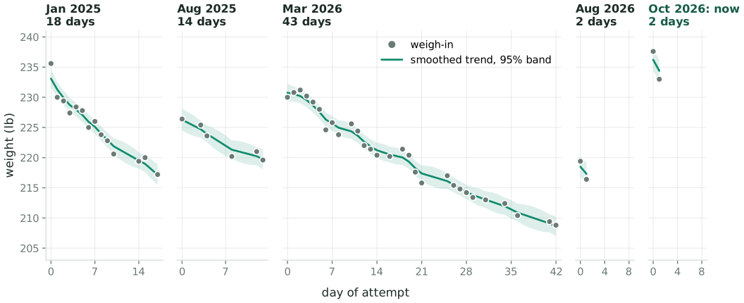
Twenty-two months on one bathroom scale
5 attemptsJan 2025 to now, months apart
73 weigh-insthe main measurement; no food log before Aug 2026, no tape before Oct 2026
±0.8 lbscatter of one morning reading about the trend, fitted from this record
7 to 22 lblost on each of the four longer attempts, then regained before the next
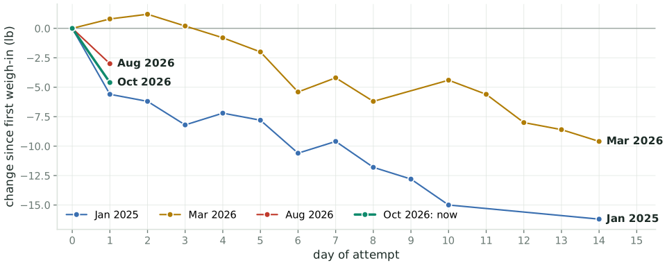
A day-one drop is mostly water
The energy budget says under 1 lb Day 1 of the current attempt: 857 kcal of metabolizable energy against roughly 3,460 kcal of expenditure, a deficit near 2,610 kcal. At about 7,800 kcal per kg of tissue that is 0.33 kg, or 0.74 lb.
The scale said 4.6 lb 237.6 → 233.0 lb overnight. The other 3.9 lb are glycogen and its bound water, gut contents, and fluid: real mass, but not the mass a diet is trying to move. A model that cannot tell the two apart will over-credit the first week and then report a “stall”.
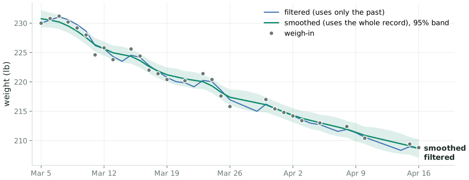
The scale is a noisy sensor of a slow state
A morning reading scatters by 0.36 kg (0.8 lb) about the true trend. That is not the scale’s error, which is tens of grams; it is fluid, gut contents, and glycogen.
Filtered: the best estimate using only readings up to that day. This is what a controller can use. Smoothed: conditioned on the whole record, the right way to review history.
Why “3,500 kcal per pound” is wrong
Mass is a mixture A lost pound is part fat (about 9,400 kcal/kg) and part lean tissue (about 1,800 kcal/kg). The mix depends on how much fat the body carries, so the energy per pound falls as the diet goes on.
Water moves first Glycogen is stored with about three times its mass in water. Cutting carbohydrate empties it in days: pounds on the scale, no tissue lost. Salt does the same in the other direction.
Expenditure adapts In a sustained deficit the body spends less than its lower mass alone explains, with a lag of a few weeks. The plateau is part of the dynamics, not a failure to comply.
Each of these is a state with its own time constant. The rest of this talk is a model with those states, a filter that estimates them from a scale, and a controller that plans food around them.
The model
Five states, nine metabolic parameters (two more with a tape measure), one equation that matters most.
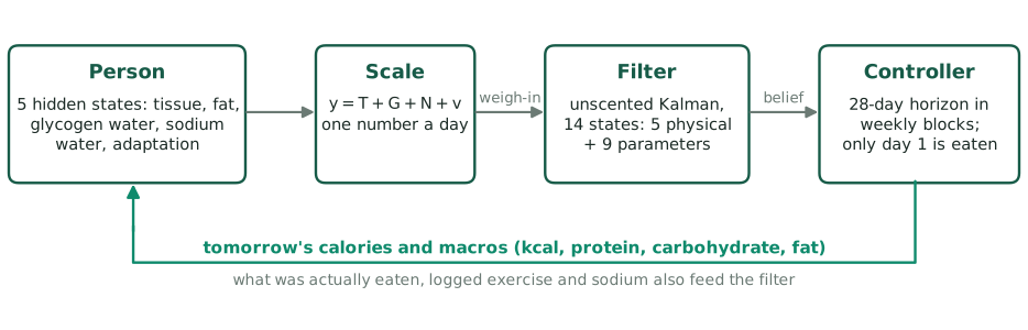
The loop
The person is a nonlinear system with five hidden states. The sensors are a scale, read each morning, and optionally a tape measure, weekly.
The filter estimates the states and the person’s metabolic parameters, jointly.
The controller plans weeks ahead from that estimate, and the subject eats only the first day of the plan. Tomorrow it plans again from a new weigh-in.
Five states
State
Units
Meaning
Clock
\(T\)
kg
tissue: fat plus fat-free solids and their water. What a diet changes
months
\(F\)
kg
fat mass, a part of \(T\) (lean mass is \(T - F\))
months
\(G_c\)
kg
glycogen and bound water, deviation from its habitual fill
1 to 2 days
\(G_n\)
kg
sodium-associated water, deviation from habitual
about 1 day
\(A\)
kcal/day
adaptive thermogenesis; negative in a deficit
about 2 weeks
\[
\rho_{\text{eff}}\,\dot T = I - E - \rho_G\,\dot G_c,
\qquad
\dot F = p\,\dot T,
\qquad
y = T + G_c + G_n + v
\]
Energy eaten \(I\) minus energy spent \(E\) goes into tissue, except what is diverted into glycogen (\(\rho_G \approx 1{,}025\) kcal/kg of glycogen-water complex). \(\rho_{\text{eff}}\) is the energy density of the tissue being lost, \(p\) its fat fraction, and the scale reads \(y\): tissue plus both water compartments plus noise \(v\).
Expenditure, and the plateau as an ODE
\[
E = c_0 + c_1 W + \text{TEF} + X + A,
\qquad
\dot A = \frac{-\beta_A\,(E_{\text{base}} - I) - A}{\tau_A}
\]
\(c_0 + c_1 W\): resting and baseline expenditure, \(W\) total mass, TEF the thermic effect of food, \(X\) logged exercise, and \(E_{\text{base}} = E - A\).
Under a sustained deficit \(D = E_{\text{base}} - I\), adaptation settles at \(-\beta_A D\) with time constant \(\tau_A\). Priors: \(\beta_A \approx 0.15\), \(\tau_A \approx 14\) days.
Water: \(\dot G_c = (k_G\,\Delta C - G_c)/\tau_G\), with \(\Delta C\) carbohydrate relative to habitual (pre-diet) intake; the same form for sodium.
Remark. \(c_0\) also absorbs any constant bias in the food log, harmlessly. A bias that drifts is another matter: the model cannot tell it apart from adaptation.
What a lost pound is made of
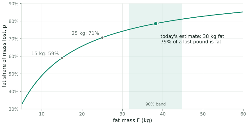
Forbes found lean mass roughly logarithmic in fat mass across people. Differentiating gives the fat share of any change:
clipped to \([0.5, 0.98]\), with \(P_g\) grams of protein. Then \(\rho_{\text{eff}} = p\,\rho_F + (1-p)\,\rho_L\).
The leaner the subject gets, the more of each pound is lean tissue, and the less energy each pound takes. The last stretch of a diet is harder than the first, structurally.
Three clocks
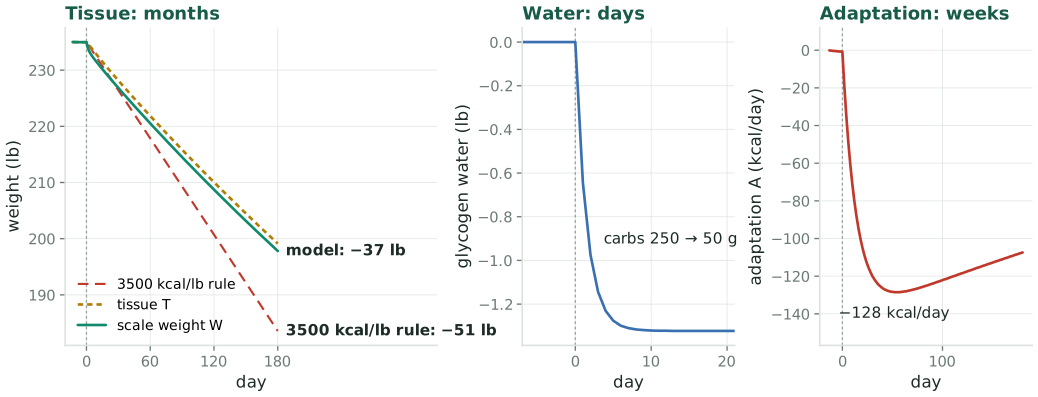
The model at its prior parameters, for a 235 lb subject who cuts 1,000 kcal/day and drops carbohydrate from 250 to 50 g on day 0. Water settles in days, adaptation in weeks, tissue in months. Over six months the model predicts 37 lb, against 51 lb for the rule of thumb.
The separation of timescales is what makes the states distinguishable at all. If adaptation were instantaneous it would be perfectly confounded with an error in \(c_0\); because it lags, a change in intake produces a brief transient in which the two differ.
From physiology to a filter
Discretize exactly Food logs are daily totals, held for a day (an exact zero-order hold) and integrated by RK4. Row \(k\) is the morning weigh-in and that day’s food, so \(x_{k+1} = f(x_k, u_k)\) takes morning \(k\) to morning \(k+1\): food never moves the reading taken before it.
Observe linearly\(y_k = H x_k + v_k\) with \(H = (1\ 0\ 1\ 1\ 0)\). The scale is linear in the state, so its update is exact. A weekly waist reading, \(a_w + b_w F\) with a personal offset and slope that are learned, is the one nonlinear update.
Unlogged days are one unknown A day with no food log sets intake to current expenditure and adds process noise along a single direction, \(\propto (1, p, 0, 0, 0)/\rho_{\text{eff}}\). An unknown intake moves tissue and fat together; diagonal noise would let the filter learn composition from nothing.
Missing weigh-ins are skipped The update is skipped and the prediction carried forward. Never interpolate a missed weigh-in by hand, and never delete an awkward one: both corrupt the noise estimate everything else rests on.
Estimation
A weight-only history identifies noise. Weight and food together identify metabolism.
Phase 1: noise, from weight alone
The first three attempts have no food log, so they cannot say anything about metabolism. They can say how noisy a reading is and how fast the trend moves. A local linear trend model does exactly that:
with level \(\ell\) and daily slope \(b\). The three noise scales are fitted by maximum likelihood over all attempts at once, each with its own diffuse start.
The record
observation sd
0.36 kg (0.8 lb)
level innovation sd
0.47 kg/day
slope innovation sd
at its bound
steady-state gain
0.71
effective window
1.4 days
Gain 0.71: each weigh-in moves the estimate 71% of the way toward itself. A standard error is reported as “unidentified” when the optimum sits on a bound, rather than as a huge number.
Unscented, not extended Sigma points go through the exact nonlinear dynamics; \(\alpha = 0.3\), because the classic \(10^{-3}\) loses positive definiteness in 14 dimensions. Smoothing is Rauch-Tung-Striebel with the sigma-point cross-covariance.
Filter in a coordinate that cannot break\(\theta = c\,e^{s\eta}\) for positive quantities, a logistic map for \(\beta_A \in (0,1)\), affine for \(\kappa_P\). Centered and scaled so the prior is exactly\(\mathcal{N}(0, I)\), and no sigma point is ever a negative time constant.
Share metabolism, not state Each attempt restarts the physical states from its first weigh-in. The parameter posterior carries over, relaxed toward the prior over two years. Attempts with no food log feed phase 1 only.
The random walk keeps the filter from going deaf to later evidence. Its cost: intervals settle at a steady width instead of shrinking forever. With a tape measure, two more slow entries carry the waist offset and slope.
Validation: does it recover what it was given?
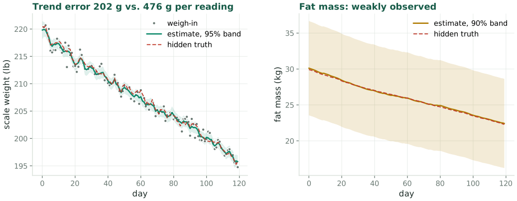
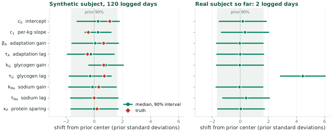
9 of 9true parameters inside their 90% intervals, truth set deliberately off the priors
205 gtrend error, from readings with 488 g of noise each
±6 kg90% band on fat mass, nearly unchanged after 120 days
Data generated by the model itself: this validates the inference machinery, and says nothing about whether the model resembles a person.
Maintenance is identified; its parts are not
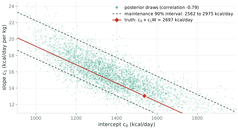
Over the narrow range of weights in one dataset, raising \(c_0\) and lowering \(c_1\) leaves the fitted trajectory almost unchanged: correlation −0.79.
So each coefficient has a wide marginal, but maintenance\(c_0 + c_1 W\) at the current weight is tight: 2,556 to 2,966 kcal/day around a true 2,697.
The package reports maintenance by propagating the full covariance through the sum. A test asserts that interval is more than 20% narrower than treating the two as independent.
What the real data has said so far
With 23 logged days, five of the nine metabolic parameters sit within half a prior standard deviation of their priors. That is the correct answer: the weigh-in history pins down noise, and nothing about metabolism, so the filter reports its ignorance instead of inventing precision.
The one that has moved most is \(\tau_{Na}\): 1.39 against a prior of 1, 0.8 prior standard deviations. From 23 logged days that is a lead, not a finding; if it is real, it will keep landing there as data accrues.
Backtest: does it forecast the scale?
Replay every attempt day by day, the filter knowing only what had happened by then; forecast the next morning’s reading, and the one a week out, from the food actually logged; score each against the scale and against persistence, “tomorrow equals the last reading”.
What synthetic tests cannot check A simulator shares the model’s assumptions, so a synthetic test cannot catch an error in them. Real weigh-ins can: food must be credited to the next morning’s reading, never the one taken before it, and attempts with no food log must feed phase 1 only, or the parameters bend to explain a deficit nobody logged.
What it says so far 22 one-day forecasts on logged days: an error of 1.4 lb against 1.8 lb for persistence. All come from the first days of a diet, when water moves most, and so few forecasts are not an evaluation. The point is that the score is recomputed at every refresh.
Control
Plan ahead, eat one day, replan.
Receding horizon
Each morning the controller takes the filtered state, optimizes intake over a horizon running to the goal date (28 days without one), prescribes the first day, and discards the rest. Tomorrow’s weigh-in corrects whatever the model got wrong.
Decisions are held constant over weekly blocks:
Per block
Bounds
energy \(I\)
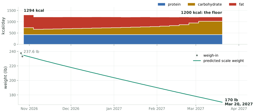
\([I_{\min}, I_{\max}]\); the subject’s floor is 1,200 kcal (default 1,500)
protein per kg
\([P_{\min}, 3.0]\) g/kg
fat share of energy
\([0.15, 0.75]\)
Carbohydrate is the residual, \(C = (I - 4P_g - 9F_g)/4\), so the three are independent and the bounds are boxes for SLSQP.
Remark. Certainty equivalence. The plan uses posterior-mean parameters and ignores their spread. That is cheap and optimistic: a maintenance estimate 200 kcal too high under-delivers, and the controller learns so only from the weigh-ins. Daily replanning keeps the error from compounding, but for the first two weeks the numbers are a starting point, not a prescription.
Not modeled: adherence. The plan is what would be optimal if followed exactly. People do not follow plans exactly.
end the horizon with less settled tissue. Linear, so it trades against the quadratic terms at an interior optimum instead of running to the floor
\(w_s\,\Delta I^2\)
do not change the target every day
\(w_e\,D^2\)
large deficits cost adherence, training and sleep, beyond any hard limit
\(w_c\,C^2\)
an optional preference for less carbohydrate, at any level
\(w_\phi(\phi - \phi^\star)^2\)
pull one macro’s energy share \(\phi\) toward a target (or break a flat tie)
\(g(z) \ge 0\)
the tissue-rate limit, every day, and the carbohydrate floor: constraints, not penalties
Settled tissue \(T^{\text{s}} = T + (\rho_G/\rho_{\text{eff}})\,G_c\) is tissue once glycogen returns to its habitual level, so neither a carbohydrate load nor a crash late in the horizon can game the score. Deadline mode replaces the progress term with tracking: settled tissue against a straight path from today’s weight to the goal, scored at the end of the horizon, not at the goal itself.
Constrain tissue, not the scale
\[
-\Delta T^{\text{s}}_k \;\le\; \frac{\gamma\, T^{\text{s}}_k}{7} \qquad \text{for every day } k
\]
\(\gamma\) is the permitted weekly tissue-loss fraction: 1.75% in the subject’s settings, 1% by default. \(T^{\text{s}}\) is settled tissue, so draining glycogen cannot loosen the limit.
Why tissue Cutting carbohydrate sheds a kilogram of glycogen water in days. On the scale that reads as 4 lb/week and trips any limit written on scale weight, though no tissue moved. A controller limited on the scale would refuse a sound plan, or raise calories in response to water. The objective scores settled tissue for the same reason: scored on \(W\), cutting carbohydrate alone would look like progress.
Constraints in fact, not intention The limit acts on the predicted trajectory, so it is a nonlinear constraint, one per day, handed to SLSQP with exact JAX Jacobians; escalating penalties survive only as a fallback. The CLI checks the final plan independently, and says so when a goal is out of reach:
target of 170 lb by 2027-01-15 is not reachable within your 1.75%/week limit; the earliest achievable date at that maximum rate is 2027-02-27
The plan being followed
1,200 kcalfirst day, November 16, 2026: 100 g protein, 155 g carbohydrate, 20 g fat
0.2 to 4.2 lb/wkpredicted scale loss; tissue at 1.6 to 1.8% of what remains a week, against the 1.75% limit
1,200 kcalthe floor, reached in week 1
Where things stand on day 22
219.9 lbfiltered trend, against a reading of 220.2: one low morning is not believed
3,133 kcalmaintenance \(c_0 + c_1W\); 90% interval 2,779 to 3,548, against the prior’s 2,200 to 3,600
33 ± 6 kgfat mass, 90%; anchored by the prior and Forbes, and by the tape (8 readings so far)
−312 kcal/dayadaptation, 22 days into a large deficit
What to expect after four months of consistent data: a trend far better than the raw scale, a personal maintenance figure good to perhaps 5 to 8% with an honest interval, a usable split of scale movement into tissue and water, and a daily plan grounded in the subject’s data rather than a population formula.
What not to expect: a reliable body-composition measurement, a trustworthy adaptation estimate unless intake is deliberately varied, or any insight into whether the plan will be followed.
What the model cannot do
Drifting log bias looks like adaptation. If under-logging grows as the weeks go by, the model sees expenditure falling. Nothing in scale data separates the two.
Intake is self-reported, and expenditure is never measured, only inferred.
Unlogged days are treated as neutral. In reality they are more often the high days.
One subject, no replication. The physiology is population-level; the fit is to one person.
Gaussian everything, and a parameter random walk that is a convenient fiction.
Reported intervals are optimistic: they assume the model is right.
Certainty-equivalent control. A stochastic or minimax formulation is the obvious extension.
Residual diagnostics can show when the model is clearly wrong. They cannot show it is right.
Remark. Not medical advice. The safety limits are conservative defaults from general guidance, not anything specific to one person.
The software
wdm, a Python package on JAX, Equinox and Diffrax:
models as JAX pytrees; RK4 one-day map, Tsit5 reference
unscented filter and smoother; phase-1 maximum likelihood
SLSQP controller, constraints on the predicted trajectory
a backtest scoring every forecast against persistence
192 tests, and a 62-page technical report deriving all of it
The daily loop, each morning before eating:
wdm daily observations.csv \--config subject.toml# asks for yesterday's food if missing,# this morning's weight, the waist# when a week has passed, and optional# health readings; then validates,# plans, logs the plan# eat the "Today:" line
Each row is a morning weigh-in plus the food eaten later that day, so this morning’s weight goes in at once and today’s food tomorrow. Every plan is archived with the command and the commit of the code that made it.
A scale is a sensor, a diet is an input, and a plateau is a time constant.
Estimate the state, respect the noise, plan ahead, act one day at a time, and let tomorrow’s weigh-in correct today’s plan.
Updated as the current attempt accrues data. Figures generated by the wdm package from the subject’s weigh-ins and food log.
The \(2n + 1\) points (29 for \(n = 14\), 33 with the tape’s two parameters) reproduce the mean and covariance exactly. Each is pushed through the one-day map, and the prediction is their weighted mean and covariance plus \(Q_k\). With \(\alpha = 10^{-3}\) and \(n \ge 14\), \(W_c^{(0)}\) is large and negative and the recombined covariance can lose positive definiteness; the package uses \(\alpha = 0.3\).
B2. The steady-state gain
Iterate the Riccati recursion of the local linear trend model to convergence and read off the Kalman gain \(K_\ell\) on the level. It answers the operational question directly: what fraction of the gap between this morning’s reading and yesterday’s estimate does the filter act on?
It is reported in place of the ratio \(\sigma_\ell/\sigma_v\), which reads as “no signal” whenever maximum likelihood drives \(\sigma_\ell \to 0\): an ordinary outcome meaning the trend moves by slope innovations rather than level jumps.
B3. Notation
Symbol
Meaning
\(T, F, G_c, G_n, A\)
tissue, fat, glycogen water, sodium water (kg); adaptation (kcal/day)
\(W = T + G_c + G_n\)
total mass, what the scale reads before noise \(v\)