Wind as a Stochastic Process: the von Karman Model
From the spectrum of the wind to the power extremum seeking loses, and the design that loses least
Robot Control Lab · Systems Engineering · UT Dallas
The published program, and what it leaves open
Rotea’s group maximizes the power of a turbine below rated wind speed by extremum seeking [R17], [CLR19], [KR22]:
- The actuator is the gain \(u\) in the generator-torque law \(\tau_g = u\Omega^2\), \(\Omega\) the rotor speed. One gain, \(u^\star\), maximizes the power.
- The probe. A sinusoid of amplitude \(a\) and period \(T\), the dither, is added to \(u\).
- The estimate. Correlating the measured log-power with the dither over one period gives \(\hat g\), an estimate of the slope of log-power with respect to \(u\).
- The step. Period after period, the gain moves along \(\hat g\) toward \(u^\star\).
- Published design for the NREL 5 MW turbine [CLR19]: \(T = 150\) s, \(a = 13.6\%\) of \(u^\star\), and a step size tuned in simulation.
What it leaves open. The wind is random, so \(\hat g\) scatters, the gain scatters about \(u^\star\) with it, and that costs power. The scatter has been measured in simulation, never predicted, so \(T\), \(a\) and the step have no rule. This deck predicts the scatter from the measured spectrum of atmospheric turbulence and chooses the \(T\), \(a\) and step that lose the least power.
What the deck derives, in order
| part | goal | result (NREL 5 MW, \(8\) m/s, turbulence intensity \(10\%\), von Karman wind) |
|---|---|---|
| Links A, B | reduce the wind’s effect on \(\hat g\) to one integral of the relative wind fluctuation | the noise in \(\hat g\) is linear in the wind |
| Links C, D | the variance of that integral, from the spectrum of turbulence | the scatter of \(\hat g\), within \(2.1\%\) of simulation, with no fitted parameter |
| The closed loop | the noise that a loop settling over many periods actually averages | the wind’s spectral density at the dither frequency, and nothing else |
| Design | the power lost as a function of \(T\), \(a\) and the tracking time, and its minimum | at a tracking time of one day, \(T = 60\) s and \(a = 10\%\) of \(u^\star\) lose \(0.23\%\) of the power; the published design loses \(0.40\%\) |
The same analysis accounts for the scatter reported in [CLR19], and it supplies the one number that a least-squares gradient estimator needs in order to report its own error bars (companion deck Least Squares for the Gradient).
Link A: reduce the randomness
Goal. Show that at the optimum the wind enters log-power through a single term, three times the relative wind fluctuation. Why. The noise in \(\hat g\) then depends on the wind through one random process, whose spectrum is measured.
What we need from the turbine
A wind turbine below rated wind speed. Write \(\bar V\) for the mean wind speed, \(R\) for the rotor radius, \(\Omega\) for the rotor angular speed, \(\rho\) for air density and \(A = \pi R^2\) for the swept area. Define the tip-speed ratio and the power coefficient:
\[\lambda := \frac{R\Omega}{V}, \qquad P = \tfrac12\rho A V^3\,C_P(\lambda)\]
\(C_P\) is a property of the blades. For the rotor studied here it has a single maximum \(C_P^{\max}\) at \(\lambda = \lambda^\star\) (the curve’s origin: A.0b). The controller’s only actuator is the torque gain \(u\) in the generator-torque law \(\tau_g = u\Omega^2\); setting \(\dot\Omega = 0\) makes the rotor rest where \(C_P(\lambda)/\lambda^3 = c\,u\) for a rotor constant \(c\) (derived in Appendix A.0), so \(u\) selects an equilibrium \(\lambda_{\text{eq}}(u)\).
Define the objective \(J(u) := \ln C_P\big(\lambda_{\text{eq}}(u)\big)\), and write \(J'\), \(J''\) for its first two derivatives in \(u\). The optimum \(u^\star\) is where \(J'(u^\star) = 0\), equivalently \(\lambda_{\text{eq}}(u^\star) = \lambda^\star\). Numerically, for the NREL 5 MW rotor at \(\bar V = 8\) m/s, \(J'' = -1.41\times10^{-13}\) in SI units.
The decomposition
Split the wind into a mean and a fluctuation about it:
\[V(t) = \bar V\big(1 + \varepsilon(t)\big), \qquad \varepsilon(t) := \frac{\tilde v(t)}{\bar V}, \qquad \mathrm{TI} := \frac{\sigma_{\tilde v}}{\bar V} = \sigma_\varepsilon\]
\(\tilde v\) is the fluctuating part in m/s, \(\varepsilon\) its dimensionless counterpart, and \(\mathrm{TI}\) the turbulence intensity, \(0.10\) in the case studied here. For a random variable \(x\), \(\sigma_x := \sqrt{\mathbb{E}[x^2] - (\mathbb{E}[x])^2}\) is its standard deviation, written \(\sigma(x)\) when \(x\) is a compound expression. For a process \(x(t)\) it is evaluated at a fixed \(t\); the assumption that makes it independent of \(t\) is stated on Link A, standing assumptions. Since \(\bar V := \mathbb{E}[V]\), both \(\tilde v\) and \(\varepsilon\) have mean zero, so \(\sigma_{\tilde v}^2 = \mathbb{E}[\tilde v^2]\) and \(\sigma_\varepsilon^2 = \mathbb{E}[\varepsilon^2]\).
Remark. The standard form is additive, \(V = \bar V + \tilde v\), with the statistics written for \(\tilde v\) [IEC]. Dividing by the constant \(\bar V\) gives the form above: \(\varepsilon = \tilde v/\bar V\) and \(\sigma_\varepsilon = \sigma_{\tilde v}/\bar V = \mathrm{TI}\).
\(\sigma_\varepsilon = 0.10\), so terms of second order in \(\varepsilon\) have typical size \(\sigma_\varepsilon^2 = 0.01\) against \(\sigma_\varepsilon = 0.10\) at first order. From here on the wind enters only through \(\varepsilon\).
Link A, executed
From the definitions, \(y = \ln P = \ln(\tfrac12\rho A) + 3\ln V + \ln C_P(\lambda)\). Substituting \(V = \bar V(1+\varepsilon)\) into the middle term, the logarithm of the product splits, and \(\ln(1+\varepsilon) = \varepsilon - \tfrac12\varepsilon^2 + O(\varepsilon^3)\) for \(|\varepsilon| < 1\):
\[3\ln V = 3\ln\bar V + 3\ln(1+\varepsilon) = \underbrace{3\ln\bar V}_{\text{constant}} + 3\varepsilon \;\underbrace{-\;\tfrac32\varepsilon^2 + O(\varepsilon^3)}_{\text{second order}}\]
The second-order part has typical size \(\tfrac32\sigma_\varepsilon^2 = 0.015\), against \(3\sigma_\varepsilon = 0.30\) for the linear term \(3\varepsilon\).
The third term, \(\ln C_P(\lambda)\), also depends on the wind, through \(\lambda = R\Omega/V\). Both wind-dependent terms are expanded under four standing assumptions, stated on the next slide; the third term is then handled on the slide after.
Link A, standing assumptions
In force through Links A and B.
- The gain is held fixed: \(u(t) = u\) on the whole interval considered. A.10 adds the dither and bounds its effect.
- \(\varepsilon\) is strictly stationary: for every \(k\), every \(s_1,\dots,s_k\) and every shift \(\tau\), the vector \((\varepsilon(s_1+\tau),\dots,\varepsilon(s_k+\tau))\) has the same joint distribution as \((\varepsilon(s_1),\dots,\varepsilon(s_k))\).
- \(\mathbb{E}[\cdot]\) is the expectation with respect to that law. For fixed \(t\), \(\mathbb{E}[\lambda(t)]\) averages the random variable \(\lambda(t)\) over the distribution of the wind. It is a number.
- The rotor has forgotten its initial condition. Linearized about its equilibrium (A.0c), the rotor equation reads \(\dot{\delta\Omega} + \delta\Omega/\tau_{\text{rotor}} = b\,\varepsilon(t)\), with \(\delta\Omega := \Omega - \Omega_{\text{eq}}\), \(\tau_{\text{rotor}} = 6.4\) s at \(8\) m/s, and \(b\) a constant (both in A.0c). Its solution from \(t = 0\) is \[\delta\Omega(t) = e^{-t/\tau_{\text{rotor}}}\,\delta\Omega(0) + b\int_0^t e^{-(t-s)/\tau_{\text{rotor}}}\,\varepsilon(s)\,ds\] The first term is deterministic and falls below \(1\%\) of \(\delta\Omega(0)\) after \(5\tau_{\text{rotor}} = 32\) s. Assumption 4 is that this has happened, so \(\Omega(t)\) is the second term alone: a causal, time-invariant functional of the wind path \(\{\varepsilon(s): s\le t\}\). The rotor still lags the wind; the lag is the exponential weight itself.
Under 1 to 4, \(V(t) = \bar V(1+\varepsilon(t))\), \(\Omega(t)\), hence \(\lambda(t) = R\Omega(t)/V(t)\) and \(y(t)\), are obtained from the wind path up to \(t\) by rules that do not change with \(t\). Assumption 2 then gives each of them the same law at every \(t\), so \(\mathbb{E}[\lambda(t)]\) and \(\mathbb{E}[y(t)]\) are constants.
Link A, executed, continued
With \(u\) fixed, \(\lambda(t)\) fluctuates only because the wind does. Write \(\bar\lambda := \mathbb{E}[\lambda(t)]\), a constant by the previous slide, and \(\delta\lambda := \lambda - \bar\lambda\). Two limits of the rotor’s response bracket \(\delta\lambda\):
- Frozen \(\Omega\). With \(\lambda_0 := R\Omega/\bar V\) and \(1/(1+\varepsilon) = 1 - \varepsilon + O(\varepsilon^2)\), \[\lambda = \frac{R\Omega}{\bar V(1+\varepsilon)} = \lambda_0\big(1 - \varepsilon + O(\varepsilon^2)\big), \qquad \bar\lambda = \lambda_0\big(1 + O(\sigma_\varepsilon^2)\big), \qquad \delta\lambda = -\bar\lambda\,\varepsilon + O(\varepsilon^2)\]
- \(\Omega\) tracking the equilibrium. \(\delta\lambda = 0\), since \(\lambda_{\text{eq}}(u)\) depends on \(u\) alone (A.0).
In both, and in between, \(\delta\lambda = O(\varepsilon)\). Expanding about \(\bar\lambda\):
\[\ln C_P(\bar\lambda + \delta\lambda) = \ln C_P(\bar\lambda) + \frac{C_P'(\bar\lambda)}{C_P(\bar\lambda)}\,\delta\lambda + O(\delta\lambda^2)\]
The next slide evaluates the two terms of this expansion at the optimum. Away from it, \(C_P'(\bar\lambda)\) is a fixed nonzero number, \(\delta\lambda = O(\varepsilon)\), and their product, the linear term, is \(O(\varepsilon)\): a fluctuation of the same order as \(3\varepsilon\), with a coefficient set by how far off the gain sits.
Link A, executed, concluded
At the optimum, \(u = u^\star\) (What we need from the turbine), so \(\lambda_{\text{eq}}(u) = \lambda^\star\), and \(d := \bar\lambda - \lambda^\star\) is a number with \(d = O(\sigma_\varepsilon^2)\) (A.0d). Three steps.
- The coefficient of the linear term. Taylor-expand \(C_P'\) about \(\lambda^\star\), where \(C_P'(\lambda^\star) = 0\) and \(C_P''(\lambda^\star) = -0.055\) is a fixed number (A.0b, continued): \[C_P'(\bar\lambda) = C_P'(\lambda^\star) + C_P''(\lambda^\star)\,d + O(d^2) = C_P''(\lambda^\star)\,d + O(\sigma_\varepsilon^4) = O(\sigma_\varepsilon^2)\]
- The linear term. \(\dfrac{C_P'(\bar\lambda)}{C_P(\bar\lambda)}\,\delta\lambda = O(\sigma_\varepsilon^2)\cdot O(\varepsilon) = O(\sigma_\varepsilon^2\,\varepsilon)\).
- The Taylor remainder. \(O(\delta\lambda^2) = O(\varepsilon^2)\), because \(\delta\lambda = O(\varepsilon)\) (previous slide).
Collecting the three terms of \(y\) from Link A, executed:
\[y = \underbrace{\ln(\tfrac12\rho A) + 3\ln\bar V + \ln C_P(\bar\lambda)}_{\text{constant}} \;+\; 3\varepsilon(t) \;+\; r(t), \qquad r := -\tfrac32\varepsilon^2 + O(\varepsilon^3) + O(\sigma_\varepsilon^2\,\varepsilon) + O(\delta\lambda^2)\]
\(\mathbb{E}[3\varepsilon] = 0\), so \(\mathbb{E}[y]\) is the constant plus \(\mathbb{E}[r]\), and \[y(t) - \mathbb{E}[y] = 3\varepsilon(t) + \big(r(t) - \mathbb{E}[r]\big)\] Every piece of \(r\) is a product of at least two factors of size \(\sigma_\varepsilon\), so \(\sigma(r - \mathbb{E}r) = O(\sigma_\varepsilon^2) \approx 0.01\) against \(\sigma(3\varepsilon) = 3\sigma_\varepsilon = 0.30\). This is what \(y - \mathbb{E}[y] = 3\varepsilon + O(\varepsilon^2)\) means wherever it is quoted below: one term, one random process.
Link B: make it a linear functional
Goal. Write the noise in \(\hat g\) as one integral of \(\varepsilon\) against the dither. Why. The variance of such an integral follows from \(\varepsilon\)’s spectrum, which is Link C.
What we need from the estimator
Extremum seeking perturbs the gain with a sinusoid of amplitude \(a\) and period \(T\). Time is cut into dither periods \([nT,(n+1)T)\), \(n = 0,1,2,\dots\); \(u_n\) is the gain about which the \(n\)-th period dithers, and the measured log-power is correlated against the sinusoid over exactly that period (written below with the period’s own clock, \(t \in [0,T]\)):
\[u(t) = u_n + a\sin\omega t, \qquad \omega := \frac{2\pi}{T}, \qquad f_1 := \frac{1}{T} = \frac{\omega}{2\pi}\]
\(\omega\) is the dither’s angular frequency (rad/s) and \(f_1\) the dither frequency in hertz; both are fixed numbers throughout, \(f_1 = 6.7\times10^{-3}\) Hz at \(T = 150\) s.
\[y(t) := \ln P(t), \qquad \hat g_n := \frac{1}{T}\int_0^T y(t)\,\frac{2}{a}\sin\omega t\;dt\]
Why that integral is a gradient estimate, and why the factor is \(2/a\), is Appendix A.1.
\(\hat g_n\) is an estimate of \(J'(u_n)\). Its mean error is the finite-amplitude bias \(\tfrac{a^2}{8}J'''\), derived on The bias grows as \(a^2\); its scatter, which is what this deck computes, comes entirely from the wind. Published values for the NREL 5 MW case [CLR19]: \(T = 150\) s and \(a = 13.6\%\) of \(u^\star\).
Link B, executed
Write the log-power over one period as three parts. \(y_0(t)\) is its value with \(\varepsilon \equiv 0\), a deterministic \(T\)-periodic function of the dither; the wind adds \(3\varepsilon(t)\) and the remainder \(r(t)\) of Link A, executed, concluded. That decomposition holds at the optimum, so Link B and everything built on it describe the estimator’s noise with the gain at \(u^\star\): the terminal scatter. (With a rotor that tracks its equilibrium it holds at every \(u\), since \(\ln C_P(\lambda_{\text{eq}}(u))\) is then constant.)
\[y(t) = y_0(t) + 3\varepsilon(t) + r(t)\]
The estimator is linear in \(y\), so it splits the same way:
\[\hat g = \underbrace{\frac{2}{aT}\int_0^T y_0\sin\omega t\,dt}_{\hat g_{\text{det}}} + \underbrace{\frac{6}{aT}\int_0^T \varepsilon(t)\sin\omega t\,dt}_{\hat g_{\text{noise}}} + \underbrace{\frac{2}{aT}\int_0^T r\sin\omega t\,dt}_{\hat g_r}\]
\(\hat g_{\text{det}}\) is a number (A.1). \(\hat g_r\) adds \(2.6\%\) to the scatter at \(\mathrm{TI} = 0.10\) (A.8); the dither’s own effect on the wind term is part of \(r\) and modulates it by at most \(10\%\) (A.10). The deck computes the scatter of the middle term:
\[\hat g_{\text{noise}} = \frac{6}{aT}\,Z, \qquad Z := \int_0^T \varepsilon(t)\,\sin\omega t\,dt\]
Link B, executed, continued
\(Z\) is a scalar random variable: the wind fluctuation over one period, weighted by the dither and integrated.
- Mean. \(\sin\omega t\) is deterministic and \(\mathbb{E}[\varepsilon(t)] = 0\) at every \(t\), so \[\mathbb{E}[Z] = \int_0^T \mathbb{E}[\varepsilon(t)]\,\sin\omega t\,dt = 0, \qquad\text{hence}\qquad \operatorname{Var}(Z) = \mathbb{E}[Z^2]\]
- \(Z^2\) as a double integral. \(Z^2 = Z\cdot Z\); name the two dummy variables \(t\) and \(s\). For a fixed realization each factor is a number independent of the other’s variable, so each moves inside the other’s integral. The iterated integral equals the double integral over \([0,T]^2\), the integrand being bounded there.
- The autocovariance. Under standing assumption 2, \(\mathbb{E}[\varepsilon(t)\varepsilon(s)]\) depends on \(t, s\) only through \(t-s\). Define \(\Gamma(t-s) := \mathbb{E}[\varepsilon(t)\varepsilon(s)]\); then \(\Gamma(0) = \sigma_\varepsilon^2\).
- Expectation inside the integral (Fubini’s theorem; its condition is checked in A.11). \[\operatorname{Var}(Z) = \mathbb{E}\!\left[\iint_{[0,T]^2}\! \sin\omega t\,\sin\omega s\;\varepsilon(t)\varepsilon(s)\,dt\,ds\right] = \iint_{[0,T]^2}\! \sin\omega t\,\sin\omega s\;\Gamma(t-s)\,dt\,ds\]
Link C: \(\operatorname{Var}(Z)\) in the frequency domain
Goal. The variance of an integral of \(\varepsilon\) against any fixed weight, from \(\varepsilon\)’s spectral density. Why. The estimator is such an integral over one period, and the loop, as shown later, is one over many periods.
The power spectral density
Standing assumption 2 (Link A, standing assumptions): \(\varepsilon\) is strictly stationary, meaning that for every \(k\), every \(s_1,\dots,s_k\) and every shift \(\tau\), \((\varepsilon(s_1+\tau),\dots,\varepsilon(s_k+\tau))\) has the same joint distribution as \((\varepsilon(s_1),\dots,\varepsilon(s_k))\). Two consequences, together called wide-sense stationarity:
- One time point (\(k = 1\) in the definition): \(\varepsilon(t)\) has the same law at every \(t\), so \(\mathbb{E}[\varepsilon] = 0\) by construction of \(\varepsilon\).
- Two time points (\(k = 2\)): shifting by \(\tau = -s\), \(\mathbb{E}[\varepsilon(t)\varepsilon(s)] = \mathbb{E}[\varepsilon(t-s)\varepsilon(0)] =: \Gamma(t-s)\), the autocovariance of Link B, executed, continued. Shifting by \(\tau\) instead, \(\Gamma(-\tau) = \mathbb{E}[\varepsilon(t)\varepsilon(t-\tau)] = \mathbb{E}[\varepsilon(t+\tau)\varepsilon(t)] = \Gamma(\tau)\): \(\Gamma\) is even.
Define, as the Fourier transform of \(\Gamma\), the power spectral density. The superscript \(2s\) marks it as two-sided: a function of every \(f \in \mathbb{R}\), negative frequencies included. Standards tabulate a one-sided version \(S\) on \(f > 0\), related on the next slide.
\[\Gamma(\tau) := \mathbb{E}\big[\varepsilon(t)\,\varepsilon(t+\tau)\big], \qquad S^{2s}(f) := \int_{-\infty}^{\infty}\! \Gamma(\tau)e^{-i2\pi f\tau}d\tau, \qquad \Gamma(\tau) = \int_{-\infty}^{\infty}\! S^{2s}(f)e^{i2\pi f\tau}df\]
The pair is the Wiener-Khinchin theorem: for \(\Gamma \in L^1(\mathbb{R})\) the transform \(S^{2s}\) exists, is real, even and nonnegative, and the inversion formula holds. Setting \(\tau = 0\) in the inversion gives \(\Gamma(0) = \sigma_\varepsilon^2 = \int S^{2s}df\). “Density” means density of variance over frequency, in units of variance per hertz: \(S^{2s}(f)\,df\) is the variance carried by frequencies in \([f, f+df]\), made precise in A.9 (a filter passing only a band leaves a process of variance \(\int_{\text{band}}S^{2s}df\)).
One-sided and two-sided densities
Frequency in hertz. Transforms are taken over \(f\) (cycles per second), with \(e^{\mp i2\pi f\tau}\) in the kernels: the turbulence standards tabulate spectra this way, and the transform pair then carries no factor \(1/2\pi\).
One-sided and two-sided. \(\Gamma\) is real and even, so \(S^{2s}\) is real and even. Tables therefore fold the negative frequencies onto the positive ones and quote the one-sided density:
\[S(f) := 2\,S^{2s}(f)\quad (f>0), \qquad\text{so}\qquad \sigma_\varepsilon^2 = \int_{-\infty}^{\infty}\!S^{2s}(f)\,df = \int_0^{\infty}\! S(f)\,df\]
Everything quoted from a standard is one-sided; every integral over all of \(\mathbb{R}\) below needs two-sided. The conversion \(S^{2s} = \tfrac12 S\) is applied once, explicitly, at the point of use.
Units: \(\varepsilon\) is dimensionless, so \([\Gamma] = 1\), \([S] = \text{Hz}^{-1}\), and \(\int S\,df\) is dimensionless.
Link C, executed
Start from Link B, \(\operatorname{Var}(Z) = \iint_{[0,T]^2}\sin\omega t\,\sin\omega s\;\Gamma(t-s)\,dt\,ds\).
- Substitute the inversion formula \(\Gamma(t-s) = \int_{\mathbb{R}} S^{2s}(f)\,e^{i2\pi f(t-s)}df\) and split the exponential, \(e^{i2\pi f(t-s)} = e^{i2\pi ft}\,e^{-i2\pi fs}\): \[\operatorname{Var}(Z) = \iint_{[0,T]^2}\sin\omega t\,\sin\omega s\int_{\mathbb{R}} S^{2s}(f)\,e^{i2\pi ft}\,e^{-i2\pi fs}\,df\,dt\,ds\]
- Move the \(f\)-integral outside (Fubini; the condition is checked below). The \(t\) and \(s\) integrals then separate: \[\operatorname{Var}(Z) = \int_{\mathbb{R}} S^{2s}(f) \left[\int_0^T\sin\omega t\,e^{i2\pi ft}dt\right]\left[\int_0^T\sin\omega s\,e^{-i2\pi fs}ds\right]df\]
- Name the brackets. Define the window \(w(t) := \sin\omega t\) for \(0 \le t \le T\) and \(w(t) := 0\) otherwise, and its Fourier transform \(\hat w(f) := \int_{\mathbb{R}} w(t)\,e^{-i2\pi ft}dt = \int_0^T\sin\omega t\,e^{-i2\pi ft}dt\) (closed form in A.3). The second bracket is \(\hat w(f)\); the first is its complex conjugate \(\overline{\hat w(f)}\), because \(w\) is real. Their product is \(|\hat w(f)|^2\): \[\boxed{\;\operatorname{Var}(Z) = \int_{\mathbb{R}} S^{2s}(f)\,|\hat w(f)|^2\,df\;}\]
- Fubini’s condition. \(\iiint|S^{2s}(f)\,\sin\omega t\,\sin\omega s\,e^{i2\pi f(t-s)}|\,dt\,ds\,df \le T^2\int_{\mathbb{R}}S^{2s}\,df = \sigma_\varepsilon^2T^2 < \infty\), using \(S^{2s} \ge 0\) and \(|\sin|, |e^{i\theta}| \le 1\).
Link C, bottom line
Result. Steps 1 to 4 used only that the weight is real, bounded and zero outside a finite interval. So for any such weight \(w\), \[\operatorname{Var}\Big(\int_{\mathbb{R}} w(t)\,\varepsilon(t)\,dt\Big) = \int_{\mathbb{R}} S^{2s}(f)\,|\hat w(f)|^2\,df\] and for one period, \(w = \sin\omega t\) on \([0,T]\), \[\sigma(\hat g_{\text{noise}}) = \frac{6}{aT}\sqrt{\int_{\mathbb{R}} S^{2s}(f)\,|\hat w(f)|^2\,df}, \qquad |\hat w(f)|^2 = \frac{4\omega^2\sin^2(\pi fT)}{(\omega^2 - 4\pi^2f^2)^2}\ \text{(A.3)}\]
- Reading. The noise variance is the wind’s density, weighted by how much of each frequency the window lets through.
- The window. An unending sine admits the frequency \(f_1\) alone. One period of it admits the band \([0, 2f_1]\), with total weight \(T/2\) (Parseval, A.3). The loop section turns on this difference.
- Needed next: \(S^{2s}\) of the actual wind, which is Link D.
- Away from \(u^\star\) the wind also enters through \(\lambda\); within the loop’s terminal scatter this changes the noise by about \(1\%\) (A.14).
Link D: the wind’s spectral density
Goal. Put in the measured spectrum of atmospheric turbulence, evaluate the variance, and check it against simulation.
The von Karman spectrum
A one-parameter model for \(S\), von Kármán’s interpolation [vK48] between the energy-containing eddies and Kolmogorov’s inertial range, listed by IEC 61400-1 [IEC] beside Kaimal and used by Lao et al. [LRKSG22]. In terms of \(\varepsilon\):
\[\boxed{\;S_\varepsilon(f) = \mathrm{TI}^2\;\frac{4L/\bar V}{\big(1+70.8\,(fL/\bar V)^2\big)^{5/6}}\;} \qquad f \ge 0,\ \text{one-sided}\]
\(L\) is the integral length scale: \(\bar V\) times the wind’s correlation time \(\int_0^\infty\Gamma(\tau)\,d\tau/\Gamma(0)\), the size of the eddies carried past the rotor. Every piece of the formula is forced or measured:
\(4L/\bar V\)
The value at \(f = 0\) that any density with integral length scale \(L\) must take (A.13).
exponent \(5/3\)
On \(f^2\), so \(S\propto (f^2)^{-5/6} = f^{-5/3}\) above the corner: Kolmogorov’s inertial-subrange law.
the \(70.8\)
Fixed by the normalization below. It places the corner, the frequency \(f = \bar V/8.41L\) at which \(70.8(fL/\bar V)^2 = 1\): below it the density is flat, above it the density falls.
It is normalized by its constant: with \(c := 70.8\) and \(x = \sqrt c\,fL/\bar V\), \(\int_0^{\infty}\! S_\varepsilon df = \tfrac{4}{\sqrt c}\int_0^\infty (1+x^2)^{-5/6}dx\,\mathrm{TI}^2 = \tfrac{2B(\frac12,\frac13)}{\sqrt c}\,\mathrm{TI}^2\), which is \(\mathrm{TI}^2\) for \(c = 4B(\tfrac12,\tfrac13)^2 = 70.78\).
Where the dither frequencies sit
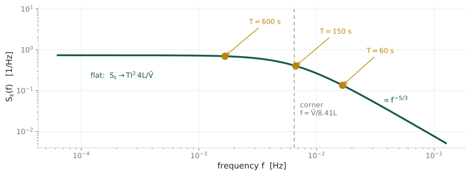
[IEC] fixes \(L\) from the hub height \(z\): \(L = 3.5\Lambda_1\) with \(\Lambda_1 = 0.7\min(z,60)\) m. For the NREL 5 MW rotor, \(z = 90\) m gives \(L = 147\) m.
At \(\bar V = 8\) m/s the corner sits at \(\bar V/8.41L = 6.5\times10^{-3}\) Hz, a period of \(155\) s, so the published \(f_1 = 1/150\) s sits on it. Above it the density falls as \(f^{-5/3}\): at \(1/150\) s it is \(3.0\) times its value at \(1/60\) s. The Design section exploits that fall.
The answer
The exact integral, evaluated numerically, against a direct simulation of the turbine under synthesized von Karman inflow, at the published \(a = 0.136\,u^\star\) (\(240\) periods per row, so a simulated \(\sigma\) carries a sampling uncertainty of about \(1/\sqrt{2\cdot240} = 4.6\%\)):
| \(T\) | \(\operatorname{Var}(Z)\) | \(\sigma(\hat g)\) predicted | \(\sigma(\hat g)\) simulated | predicted/simulated |
|---|---|---|---|---|
| \(150\) s | \(17.04\) | \(5.43{\times}10^{-7}\) | \(5.51{\times}10^{-7}\) | \(0.986\) |
| \(300\) s | \(46.53\) | \(4.49{\times}10^{-7}\) | \(4.58{\times}10^{-7}\) | \(0.981\) |
| \(600\) s | \(104.9\) | \(3.37{\times}10^{-7}\) | \(3.44{\times}10^{-7}\) | \(0.979\) |
\[\boxed{\;\sigma(\hat g) = \frac{6}{aT}\sqrt{\int_{\mathbb{R}}\tfrac12 S_\varepsilon(f)\,|\hat w(f)|^2\,df}\;}\] Within \(2.1\%\) of simulation across a fourfold range of \(T\), with no fitted parameter: \(\mathrm{TI}\), \(L\) and the exponent \(5/3\) come from the standard and from turbulence theory, \(T\) and \(a\) from the published design. In units of the gain, \(\sigma(\hat g)/|J''| = 1.7\,u^\star\) at \(T = 150\) s: one period’s estimate is far too noisy to step on alone, and the loop reaches a scatter of a few percent of \(u^\star\) only by averaging over many periods (next section).
Every link holds
The turbine is integrated with an adaptive solver under synthesized von Karman inflow (A.12): \(240\) periods of \(T = 150\) s at \(\bar V = 8\) m/s, with realized turbulence intensity \(9.87\%\) and the gain held at \(u^\star\) so that the estimator is tested alone. Each link is tested separately, so that a failure can be attributed.
| link | claim | test | predicted | measured | ratio |
|---|---|---|---|---|---|
| A | \(y-\mathbb{E}[y] = 3\varepsilon\) | regress \(y\) on the recorded \(\varepsilon\) | slope \(3\) | slope \(3.087\), \(r = 0.9918\) | \(1.037\) |
| C | \(\operatorname{Var}Z = \int S^{2s}\vert\hat w\vert^2 df\) | sample variance of \(Z\) | \(17.04\) | \(16.61\) | \(0.975\) |
| D | \(\sigma(\hat g) = \tfrac{6}{aT}\sqrt{\operatorname{Var}Z}\) | sample deviation of \(\hat g\) | \(5.43{\times}10^{-7}\) | \(5.51{\times}10^{-7}\) | \(1.014\) |
All three within \(5\%\). Link B is algebra given A, \(\hat g_{\text{noise}} = \tfrac{6}{aT}Z\) by linearity of the estimator, and is tested through D. The ratio on A is \(\sigma(y)/\sigma(3\varepsilon)\).
Every link holds, continued
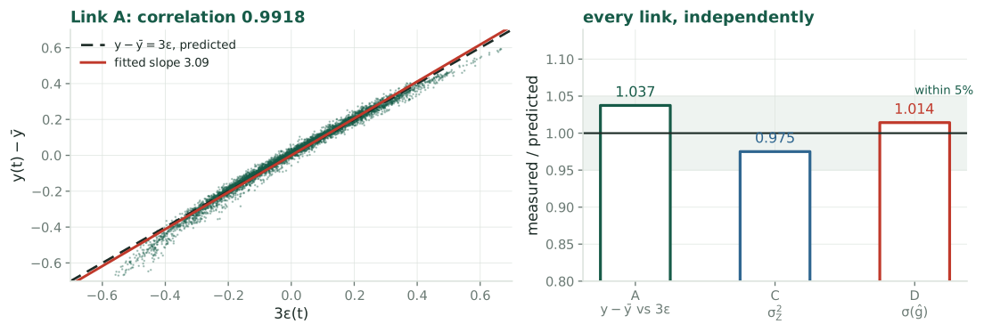
- The \(3.7\%\) on A. The slope exceeds \(3\) by \(2.9\%\): the \(O(\sigma_\varepsilon^2\varepsilon)\) term of Link A, executed, concluded, \(\kappa_2\sigma_\varepsilon^2\varepsilon = 0.063\,\varepsilon\) for a frozen rotor and \(0\) for a tracking one. The rest is the remainder uncorrelated with \(\varepsilon\), \(\sqrt{1-r^2} = 13\%\) of \(\sigma(y)\): \(\sqrt{1.029^2 + 0.128^2} = 1.037\).
- Row D compares the total scatter, remainder included, with the prediction for \(\hat g_{\text{noise}}\) alone: the remainder adds \(2.7\%\) (A.8) and Link C’s sample falls \(2.5\%\) short, \(1.027\times\sqrt{0.975} = 1.014\).
The closed loop
Goal. The loop steps on hundreds of estimates before it settles. Find the noise it actually averages, and the scatter it leaves in the gain: that scatter is what costs power.
The bias grows as \(a^2\)
Link B wrote \(\hat g = \hat g_{\text{det}} + \hat g_{\text{noise}} + \hat g_r\). Both wind-driven parts have mean zero, \(\mathbb{E}[Z] = 0\) and \(\mathbb{E}[\hat g_r] = \tfrac{2}{aT}\mathbb{E}[r]\int_0^T\sin\omega t\,dt = 0\), so \(\mathbb{E}[\hat g] = \hat g_{\text{det}}\) and the bias is \(\operatorname{Bias} := \hat g_{\text{det}} - J'(u)\). By A.1, \(\hat g_{\text{det}} = \tfrac{2}{aT}\int_0^T J(u + a\sin\omega t)\sin\omega t\,dt\).
With \(s := \sin\omega t\), \(\langle\cdot\rangle := \tfrac1T\int_0^T(\cdot)\,dt\), and the moments of a sine over a whole period (A.2),
\[\langle s\rangle = 0,\qquad \langle s^2\rangle = \tfrac12,\qquad \langle s^3\rangle = 0,\qquad \langle s^4\rangle = \tfrac38\]
expand \(J(u + as) = J + J'as + \tfrac{J''}{2}a^2s^2 + \tfrac{J'''}{6}a^3s^3 + O(a^4)\), multiply by \(\tfrac{2}{a}s\) and average:
\[\hat g_{\text{det}} = \frac2a\Big[J\langle s\rangle + J'a\langle s^2\rangle + \tfrac{J''}{2}a^2\langle s^3\rangle + \tfrac{J'''}{6}a^3\langle s^4\rangle\Big] + O(a^4) = J' + \frac{a^2}{8}J''' + O(a^4)\]
\[\operatorname{Bias}(\hat g) = \frac{a^2}{8}\,J'''(u) + O(a^4), \qquad \sigma(\hat g_{\text{noise}}) = \frac{6}{aT}\,\sigma(Z) \propto \frac1a\] The bias grows with the probe; the scatter falls with it, because \(Z\) does not involve \(a\). Checked numerically on a cubic \(J\), where \(J'''\) is exact: agreement to six digits at \(a = 0.02\), \(0.05\), \(0.10\).
The closed loop
- The update. \(u_{n+1} = u_n + \kappa\,\hat g_n\), with a constant step \(\kappa > 0\) and \(\tilde u_n := u_n - u^\star\).
- The mean of \(\hat g_n\) near \(u^\star\). \(J'(u_n) = J''\tilde u_n + O(\tilde u_n^2)\) with \(J'' < 0\). The rotor follows the dither with a lag, which scales the part of the power in phase with the dither by (A.0c, continued) \[G_1 := \frac{1}{1 + (2\pi\tau_{\text{rotor}}/T)^2}:\qquad \mathbb{E}[\hat g_n] = G_1\big(J''\tilde u_n + \operatorname{Bias}\big)\] \(G_1 = 0.93\) at \(T = 150\) s and \(0.69\) at \(60\) s. The bias shifts the fixed point to \(\tilde u = -a^2J'''/(8J'')\) and is set aside here.
- The recursion. With \(K := \kappa\,G_1|J''|\), the fraction of the error removed per period, \[\tilde u_{n+1} = (1-K)\,\tilde u_n + \kappa\,e_n, \qquad e_n := \hat g_{\text{noise},n} + \hat g_{r,n}\]
- Its stationary variance (A.4), with \(\rho_k\) the correlation between estimates \(k\) periods apart (A.6): \[\operatorname{Var}(\tilde u) = \frac{\kappa^2\sigma^2(\hat g)}{K(2-K)}\Big[1 + 2\sum_{k\ge1}(1-K)^k\rho_k\Big]\]
Two regimes. A fast loop, \(K\) near \(1\), weights only \(k = 0\): one period’s \(\sigma(\hat g)\) sets the scatter. A slow loop, \(K \ll 1\), has \((1-K)^k \approx 1\) wherever \(\rho_k\) is nonzero, and the bracket tends to \(1 + 2\sum_{k\ge1}\rho_k\): the scatter is set by the long-run variance \(\sigma_\infty^2(\hat g) := \sigma^2(\hat g)\big[1 + 2\sum_{k\ge1}\rho_k\big]\), and \(\operatorname{Var}(\tilde u) \approx \tfrac{K}{2}\,\sigma_\infty^2(\hat g)/(G_1J'')^2\).
The noise a slow loop averages
Goal: \(\sigma_\infty^2\) in closed form. Route: the mean of \(N\) consecutive estimates is a single estimate over a window \(N\) periods long, and Link C gives its variance.
- The mean of \(N\) estimates is one window. The dither \(\sin\omega t\) runs on across period boundaries, so \[\bar{\hat g}_N := \frac1N\sum_{n=0}^{N-1}\hat g_n = \frac{2}{aNT}\int_0^{NT}y(t)\sin\omega t\,dt, \qquad \text{noise part } \frac{6}{aNT}\int_0^{NT}\varepsilon(t)\sin\omega t\,dt\]
- Its variance, by Link C with the window \(w_N := \sin\omega t\) on \([0, NT]\) (A.3): \[\operatorname{Var}(\bar{\hat g}_N) = \Big(\frac{6}{aNT}\Big)^2\int_{\mathbb{R}} S^{2s}(f)\,|\hat w_N(f)|^2\,df, \qquad |\hat w_N(f)|^2 = \frac{4\omega^2\sin^2(\pi fNT)}{(\omega^2 - 4\pi^2f^2)^2}\]
- The window narrows onto \(\pm f_1\). Its total area is \(NT/2\) (Parseval, A.3). Away from \(\pm f_1\) it stays below \(4\omega^2/(\omega^2 - 4\pi^2f^2)^2\), a bound free of \(N\), so as \(N\) grows its area gathers at \(\pm f_1\), \(NT/4\) at each: \(\int S^{2s}|\hat w_N|^2df = S^{2s}(f_1)\,NT/2 + o(N)\).
- Multiply by \(N\) and let \(N \to \infty\). By A.7, \(N\operatorname{Var}(\bar{\hat g}_N) \to \sigma_\infty^2(\hat g)\). Hence \[\boxed{\;\sigma_\infty^2(\hat g) = \lim_{N\to\infty}N\Big(\frac{6}{aNT}\Big)^2S^{2s}(f_1)\,\frac{NT}{2} = \frac{2R}{a^2T}, \qquad R := 9\,S^{2s}(f_1)\;}\] \(R\) is the two-sided density, at the dither frequency, of the wind’s term \(3\varepsilon\) in log-power.
The noise a slow loop averages, continued
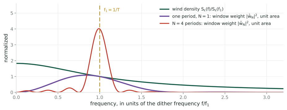
- One period (violet) admits the band \([0, 2f_1]\), and below \(f_1\) the density (green) rises to \(1.8\) times its value at \(f_1\): one period’s variance exceeds the long-run value, by less than under Kaimal, whose density rises \(5.2\) times. Four periods (red) already admit little beyond \(f_1\).
- In time: adjacent estimates correlate at \(\rho_1 = -0.06\) (\(T = 150\) s, A.6), so their low-frequency parts cancel in the average. \(\sigma_\infty^2/\sigma^2(\hat g) = 0.68\), \(0.88\), \(1.00\) at \(T = 60\), \(150\), \(600\) s.
Checked: the scatter of the loop
The linearized loop of The closed loop, driven period by period by \(Z_n\) from synthesized von Karman wind (A.12), with \(a = 0.136\,u^\star\) and \(K = T/86\,400\) s (the loop forgets its state in one day); \(24\) records of \(20\) days per row, so a measured \(\sigma(\tilde u)\) carries a sampling uncertainty of about \(3.5\%\):
| \(T\) | \(\sigma(\tilde u)/u^\star\) measured | predicted from \(\sigma_\infty\) | predicted from one period’s \(\sigma\) | long-run variance of \(Z\): measured / \(S^{2s}(f_1)T/2\) |
|---|---|---|---|---|
| \(60\) s | \(0.0288\) | \(0.0278\) | \(0.0337\) | \(1.993\) / \(2.025\) |
| \(150\) s | \(0.0475\) | \(0.0479\) | \(0.0510\) | \(14.84\) / \(15.08\) |
| \(600\) s | \(0.0596\) | \(0.0632\) | \(0.0633\) | \(98.65\) / \(104.5\) |
The long-run prediction holds to within \(4\%\) at \(60\) and \(150\) s, where one period’s variance overstates the scatter by \(17\%\) and \(7\%\). On the full nonlinear turbine in closed loop (\(K = 0.015\), \(T = 600\) s, \(270\) periods) the measured scatter is \(0.77\) of the prediction, against \(0.79\) expected from so short a record (A.5).
Design
Goal. Choose the period, the amplitude and the step so that the loop loses the least power while still tracking the optimum in a required time.
Design, the objective: Power lost, in two parts
- Loss in terms of \(J\). \(J = \ln C_P\), so \(J(u^\star) - J\) is the relative power loss at the operating point (for a small loss, \(-\ln(1-x) \approx x\)).
- What the rotor sees. The gain is \(u^\star + \tilde u + a\sin\omega t\). The rotor follows the slow \(\tilde u\) fully and the dither through its lag, which scales the dither’s effect on \(\lambda\) by \(|G| = \sqrt{G_1}\) and delays it by \(\varphi\) (A.0c, continued). So \(\lambda\) sits at \(\lambda_{\text{eq}}\big(u^\star + \tilde u + a\sqrt{G_1}\sin(\omega t - \varphi)\big)\).
- Expand about \(u^\star\), where \(J' = 0\): \[J(u^\star) - J = \tfrac12|J''|\big(\tilde u + a\sqrt{G_1}\sin(\omega t-\varphi)\big)^2 + O\big((\tilde u + a)^3\big)\]
- Average over the wind (\(\mathbb{E}[\tilde u] = 0\) at the fixed point, up to the bias shift) and over one period (\(\langle\sin^2\rangle = \tfrac12\), \(\langle\sin\rangle = 0\)): \[\boxed{\;\text{loss} = \tfrac12|J''|\operatorname{Var}(\tilde u) + \tfrac14|J''|\,G_1a^2\;}\] the first term from the gain wandering about \(u^\star\), the second from the dither itself.
- Scale. \(|J''|u^{\star2} = 0.70\) (NREL 5 MW), so \(\sigma(\tilde u) = 0.10\,u^\star\) costs \(0.35\%\), and \(a = 0.136\,u^\star\) at \(T = 150\) s costs \(0.30\%\).
Design, the requirement: How fast must the loop track?
- What moves \(u^\star\). \(\lambda_{\text{eq}}(u)\) involves \(u\) and the blades only (A.0), so \(u^\star\) is the same at every mean wind speed. It moves only when the blades change, by erosion, icing or fouling, over weeks [KR24].
- When the loop must re-converge: after start-up, and after a spell above rated wind speed with the loop paused. Both are events of order a day.
- Tracking time. The error forgets its initial value as \((1-K)^n \approx e^{-nK}\), that is, in \(\tau_c := T/K\) seconds. Adopted here: \(\tau_c = 1\) day \(= 86\,400\) s, so \(K = T/\tau_c = 0.0007\) at \(T = 60\) s and \(0.0017\) at \(150\) s: a slow loop.
- The scatter at that tracking time. From The closed loop with \(\kappa = K/(G_1|J''|)\) and \(\sigma_\infty^2 = 2R/(a^2T)\): \[\operatorname{Var}(\tilde u) = \frac K2\,\frac{\sigma_\infty^2(\hat g)}{G_1^2J''^2} = \frac{T}{2\tau_c}\cdot\frac{2R}{a^2T}\cdot\frac{1}{G_1^2J''^2} \;\Longrightarrow\; \boxed{\;\operatorname{Var}(\tilde u) = \frac{R}{a^2\,G_1^2\,\tau_c\,J''^2}\;}\]
At a fixed tracking time the period enters only through \(R(T) = 9\,S^{2s}(1/T)\), the wind’s density at the dither frequency, and through the rotor’s \(G_1(T)\).
Design, the amplitude: The two losses balance
- Loss as a function of \(a\), from the two previous slides: the first term falls as \(1/a^2\), the second rises as \(a^2\), \[\text{loss}(a) = \frac{R}{2a^2G_1^2\tau_c|J''|} + \tfrac14|J''|\,G_1a^2\]
- Minimize. \(d\,\text{loss}/da = -R/(a^3G_1^2\tau_c|J''|) + \tfrac12|J''|G_1a = 0\) gives \(a_{\text{opt}}^4 = 2R/(G_1^3\,\tau_c\,J''^2)\), at which the two terms are equal.
- The least loss is therefore twice the second term: \[\boxed{\;\text{loss}_{\min} = \tfrac12|J''|\,G_1a_{\text{opt}}^2 = \sqrt{\frac{R}{2\,\tau_c\,G_1}}\;}\] free of \(J''\): the curvature sets where the optimum lies, not what it costs.
| \(T\) | \(a_{\text{opt}}/u^\star\) | \(\sigma(\tilde u)/u^\star\) | \(\text{loss}_{\min}\) |
|---|---|---|---|
| \(60\) s | \(0.096\) | \(0.057\) | \(0.23\%\) |
| \(150\) s | \(0.101\) | \(0.069\) | \(0.33\%\) |
| \(600\) s | \(0.111\) | \(0.078\) | \(0.43\%\) |
The bias shift, \(-a^2J'''/(8J'') = 0.20\,(a/u^\star)^2u^\star\) from \(J'''u^{\star3} = 1.13\), is \(0.002\,u^\star\) at \(a_{\text{opt}}\): negligible.
Design, the period: Short, until the rotor’s lag takes over
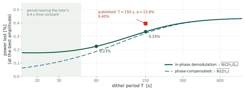
\(\text{loss}_{\min} \propto \sqrt{R/G_1}\). From \(150\) s to \(60\) s the density \(R\) falls \(3.0\) times while \(G_1\) falls only from \(0.93\) to \(0.69\): the loss drops from \(0.33\%\) to \(0.23\%\).
Design, the period, continued: Where to stop
- The curve flattens below \(45\) s: \(0.20\%\) at \(45\) s, \(0.18\%\) at its minimum near \(19\) s. There the period nears the rotor’s \(6.4\) s time constant, where the static \(C_P(\lambda)\) curve and the first-order rotor model on which this section rests are least reliable (the wake’s induction also lags, on a time of order \(R/\bar V = 8\) s).
- \(T = 60\) s takes most of the gain with a margin of ten rotor time constants.
- Phase compensation (dashed curve). Demodulate against the dither delayed by the rotor’s phase lag \(\varphi\) (A.0c, continued): \[\hat g_{\text{pc}} := \frac{2}{aT}\int_0^T y\,\sin(\omega t - \varphi)\,dt \;\to\; J'\sqrt{G_1}, \qquad \varphi = \arctan\frac{2\pi\tau_{\text{rotor}}}{T}\] instead of \(J'G_1\). The long-run noise is the same, so \(G_1\) leaves the loss: \(\sqrt{R/(2\tau_c)} = 0.19\%\) at \(T = 60\) s. It needs \(\tau_{\text{rotor}}\), which scales as \(1/\bar V\) (A.0c).
Design, the step size: From the design curve
- The step follows from \(K = T/\tau_c\): \(\kappa = K/(G_1|J''|)\), evaluated at \(u^\star\).
- \(J''\) is a property of the blades. \(J(u) = \ln C_P(\lambda_{\text{eq}}(u))\) with \(\lambda_{\text{eq}}\) from \(C_P(\lambda)/\lambda^3 = c\,u\) (A.0): the same function at every wind speed, with \(J''(u^\star) = -1.41\times10^{-13}\) in SI units, computed once from the design curve.
- Its variation along the curve. \(J''(u)/J''(u^\star) = 2.0\) at \(0.7u^\star\), \(1.2\) at \(0.9u^\star\), \(0.79\) at \(1.2u^\star\), \(1.6\) at \(2u^\star\). Within the terminal scatter, \(|\tilde u| \lesssim 0.1u^\star\), it stays within \(\pm20\%\); far from \(u^\star\), during the transient, the step is off by up to a factor \(2\), which a tracking time of a day absorbs.
Rule. \(\kappa = T/\big(\tau_c\,G_1\,|J''(u^\star)|\big)\), with no tuning and no online curvature estimate. If the blades degrade, re-estimate \(|J''|\) on the weeks-long time scale on which they change (A.15).
Design, the published loop
| published [CLR19] | derived here | |
|---|---|---|
| period \(T\) | \(150\) s | \(60\) s |
| amplitude \(a\) | \(13.6\%\) of \(u^\star\) | \(9.6\%\) of \(u^\star\) |
| step \(\kappa\) | tuned in simulation | \(T/(\tau_c\,G_1\,\vert J''(u^\star)\vert)\) |
| power lost, tracking time one day | \(0.40\%\) | \(0.23\%\) |
The published scatter. [CLR19] reports a tip-speed-ratio scatter \(\sigma(\lambda) \lesssim 0.14\). Since \(d\ln\lambda_{\text{eq}}/d\ln u = -1/3\) at \(u^\star\) (A.10), \[\sigma(\lambda) = \tfrac13\lambda^\star\,\sigma(\tilde u)/u^\star\] and at the published \(T\) and \(a\):
- a loop settling in three periods (\(K = 0.5\)) would give \(\sigma(\lambda) = 2.6\), \(19\) times the report;
- a loop with \(\tau_c = 1\) day gives \(0.13\), and \(\tau_c = 20\) h gives \(0.14\).
The published scatter implies a loop that averages over most of a day. The paper’s loop gain, which it does not report, would settle the question.
Bottom line
- The scatter of one period’s estimate follows from \(\mathrm{TI}\), \(L\) and \(\bar V\) alone, \(\sigma(\hat g) = \tfrac{6}{aT}\sqrt{\int S^{2s}|\hat w|^2df}\), within \(2.1\%\) of simulation.
- A slow loop averages less noise, set by the wind’s density at the dither frequency alone: \(\sigma_\infty^2 = 2R/(a^2T)\), \(R = 9\,S^{2s}(f_1)\).
- The least power lost at tracking time \(\tau_c\) is \(\sqrt{R/(2\tau_cG_1)}\). \(T \approx 60\) s and \(a_{\text{opt}} \approx 10\%\) of \(u^\star\) reach it: \(0.23\%\) against \(0.40\%\) for the published design.
- The step follows from the design curve, \(\kappa = T/(\tau_cG_1|J''(u^\star)|)\).
- Two further levers. Phase-compensated demodulation, \(0.19\%\) at \(60\) s. And subtracting \(3\ln(\hat V/\bar V)\) from a wind measurement \(\hat V\) (nacelle anemometer, lidar) whose coherence with the rotor’s wind at \(f_1\) is \(\varrho\): this multiplies \(R\) by \(1 - \varrho^2\) and the loss by \(\sqrt{1-\varrho^2}\).
Two models of the spectrum
Goal. IEC 61400-1 offers two densities for the longitudinal wind, Kaimal and von Karman. Compare them, and carry the difference through to the noise and the design. The same analysis is worked out under each: Kaimal · von Karman.
Two models: the formulas
Both are one-sided densities of \(\varepsilon\) with the A.13 prefactor; Lao et al. [LRKSG22], eq. (18), use the second:
\[S^{\mathrm{K}}_\varepsilon(f) = \mathrm{TI}^2\;\frac{4L/\bar V}{\big(1+6fL/\bar V\big)^{5/3}}, \qquad S^{\mathrm{vK}}_\varepsilon(f) = \mathrm{TI}^2\;\frac{4L/\bar V}{\big(1+70.8\,(fL/\bar V)^2\big)^{5/6}}\]
| Kaimal [KWIC72] | von Karman [vK48] | |
|---|---|---|
| value at \(f = 0\) | \(4L\,\mathrm{TI}^2/\bar V\) | \(4L\,\mathrm{TI}^2/\bar V\) |
| above the corner | \(\propto f^{-5/3}\) | \(\propto f^{-5/3}\) |
| \(\int_0^\infty S\,df\) | \(\mathrm{TI}^2\) | \(\mathrm{TI}^2\) (\(70.8\) is \(70.78\) rounded, the value that makes it exact) |
| IEC length, hub \(\ge 60\) m | \(L = 8.1\Lambda_1 = 340\) m | \(L = 3.5\Lambda_1 = 147\) m (Lao et al.: \(150\) m) |
| corner at \(\bar V = 8\) m/s | \(\bar V/6L = 0.0039\) Hz | \(\bar V/(8.41L) = 0.0065\) Hz |
- One family. Both are the A.13 prefactor times a shape that is flat below a corner and falls as Kolmogorov’s \(f^{-5/3}\) above it. They differ in how the corner is turned.
- Different \(L\), on purpose. IEC picks the two lengths so that the \(f^{-5/3}\) ranges coincide: at \(1\) Hz the densities agree to \(0.2\%\). The price is the low end. The models disagree on the integral length scale itself (\(340\) against \(147\) m), and so on \(S(0)\), by a factor of \(2.31\).
Two models: where the dither frequencies sit
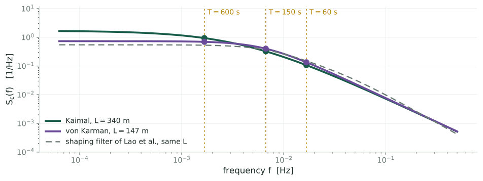
The design reads each density at \(f_1\) only. Kaimal over von Karman there: \(1.35\) at \(T = 600\) s, \(1.03\) at \(314\) s, \(0.81\) at \(150\) s, \(0.79\) at \(60\) s. The published \(150\) s sits just above Kaimal’s corner and on von Karman’s.
Two models: what changes downstream
Links A to C never use the form of \(S\). Link D and the closed loop read it at \(f_1\), through \(S^{2s}(f_1)\,T/2\), so the choice enters as one ratio per period:
| \(T\) | \(S^{\mathrm{K}}(f_1)/S^{\mathrm{vK}}(f_1)\) | \(\sigma(\tilde u)/u^\star\), Kaimal | \(\sigma(\tilde u)/u^\star\), von Karman | measured ratio | \(\sqrt{S^{\mathrm{K}}/S^{\mathrm{vK}}}\) |
|---|---|---|---|---|---|
| \(60\) s | \(0.794\) | \(0.0257\) | \(0.0288\) | \(0.892\) | \(0.891\) |
| \(150\) s | \(0.808\) | \(0.0427\) | \(0.0475\) | \(0.899\) | \(0.899\) |
| \(600\) s | \(1.353\) | \(0.0693\) | \(0.0596\) | \(1.163\) | \(1.163\) |
The loop of Checked: the scatter of the loop, run on both synthesized winds (same seeds, \(24\) records of \(20\) days per row). At the design level (\(\tau_c = 1\) day):
| Kaimal | von Karman | |
|---|---|---|
| least loss at \(T = 60\) s, \(a_{\text{opt}}\) | \(0.20\%\), \(a = 9.1\%\) of \(u^\star\) | \(0.23\%\), \(a = 9.6\%\) of \(u^\star\) |
| published design (\(150\) s, \(13.6\%\)) | \(0.38\%\) | \(0.40\%\) |
Changing the model changes no derivation; it rescales the scatter at each \(T\) by \(\sqrt{S(f_1)}\), exactly as The noise a slow loop averages says it must. Kaimal is the noisier model at \(T = 600\) s, von Karman by \(11\) to \(12\%\) at the short periods. The design rule and its choice of \(T = 60\) s survive the change of model; the loss it achieves moves by \(0.02\) points.
Two models: the shaping filter of Lao et al.
Lao et al. do not synthesize from eq. (18). They pass unit white noise through a rational filter and scale its output by \(\sigma = I\,V_m\) [LRKSG22], eqs. (19)–(21):
\[H_t(s) = \frac{K_F\,(m_1T_Fs+1)}{(T_Fs+1)(m_2T_Fs+1)},\qquad T_F = \frac{L}{V_m},\quad K_F = \sqrt{\frac{2\pi T_F}{B(\tfrac12,\tfrac13)}},\quad m_1 = 0.4,\ m_2 = 0.25\]
- Why a filter. The exponents \(5/6\) and \(5/3\) are not integers, so no finite-order linear system has exactly the von Karman density; a filter is needed to generate the wind online, sample by sample. A.12 builds the whole record at once and evaluates \(S\) exactly on its frequency grid, so it needs no filter.
- The variance is right. For white noise of two-sided density \(1\) the output variance is \(0.98\,\sigma^2\): \(K_F\) is the normalization.
- The shape is approximate. Their filter’s density against eq. (18), at their \(L = 150\) m, \(V_m = 12\) m/s (\(T_F = 12.5\) s):
| \(f\) | \(0\) | \(1/600\) Hz | \(1/150\) Hz | \(1/60\) Hz | \(0.08\) Hz (\(fT_F = 1\)) | \(1\) Hz |
|---|---|---|---|---|---|---|
| \(S_{H_t}/S^{\mathrm{vK}}\) | \(0.75\) | \(0.75\) | \(0.84\) | \(1.02\) | \(1.37\) (largest) | \(0.73\) |
Above the corner the filter falls as \(f^{-2}\), not \(f^{-5/3}\), so the ratio keeps falling as \(f^{-1/3}\).
For ten-minute constraint tests, which is what Lao et al. need, the variance is what matters and the filter gets it right. For this analysis, whose noise is \(S(f_1)\), the filter’s error at the dither frequency (\(0.75\) to \(1.02\)) is as large as the gap between Kaimal and von Karman themselves, which is why A.12 synthesizes from the spectrum directly.
Appendices
The derivations the main line cites.
A.0: Where the equilibrium relation comes from
The rotor is a rigid body of inertia \(I\), driven by aerodynamic torque and braked by the generator: \(I\dot\Omega = \tau_{\text{aero}} - \tau_g\) with \(\tau_g = u\Omega^2\). Power is torque times angular speed, and \(\Omega = \lambda V/R\), so with \(A = \pi R^2\)
\[\tau_{\text{aero}} = \frac{P}{\Omega} = \frac{\tfrac12\rho\pi R^2V^3C_P(\lambda)}{\lambda V/R} = \tfrac12\rho\pi R^3V^2\,\frac{C_P(\lambda)}{\lambda}\]
At rest \(\dot\Omega = 0\), so \(\tau_{\text{aero}} = \tau_g = u\lambda^2V^2/R^2\). The \(V^2\) on the two sides cancels, and dividing through:
\[\boxed{\;\frac{C_P(\lambda)}{\lambda^3} = \frac{2}{\rho\pi R^5}\,u =: c\,u\;}\]
A curve set by the blades meets a line set by the gain at \(\lambda_{\text{eq}}(u)\), and \(V\) is gone. That cancellation is the reason for the \(\Omega^2\) law: any other power of \(\Omega\) leaves a factor of \(V\) behind.
\(C_P/\lambda^3\) is not monotone. For the curve of A.0b it falls from \(+\infty\) (the fit is linear in \(\lambda\) near \(0\)) to a minimum at \(\lambda = 2.25\), rises to a maximum at \(3.95\), then falls. Rest points are stable where it falls. For \(u < 1.86\,u^\star\) the only root is on the branch through \(\lambda^\star\); \(\lambda_{\text{eq}}(u)\) means that root.
A.0b: Where the shape of \(C_P(\lambda)\) comes from
Three layers, from what is a theorem down to what is a fit.
physics fixes the envelope
\(C_P \ge 0\), and \(C_P \le 16/27 \approx 0.593\) for any rotor: the Betz limit, from momentum conservation on the stream tube alone. At \(\lambda \to 0\) the rotor is stopped and extracts nothing; at large \(\lambda\) the blades run faster than the wind can feed them and drag dominates. So \(C_P\) must rise from zero and fall back, and has at least one maximum.
blade design fixes the curve
For a given blade, \(C_P(\lambda)\) is computed by blade-element momentum theory: slice the blade spanwise, look up each section’s lift and drag against its local angle of attack from wind-tunnel airfoil tables, integrate. The result is empirical in its inputs and deterministic in its arithmetic. For a well-designed blade at fixed pitch it has one peak.
what this deck uses
Heier’s closed-form fit to typical BEM curves [H98], remapped so its maximum sits at \((\lambda^\star, C_P^{\max}) = (7.5,\,0.49)\), the design values of the NREL 5 MW rotor from [J09]. A stand-in with the right peak and the right asymmetry, steep on the stall side and gentle above.
So “single maximum” is an empirical property of good blades, and the specific curve here is a fit. Two consequences the main line depends on survive any such curve: \(C_P' = 0\) at the maximum \(\lambda^\star\), which is what Link A uses, and \(C_P/\lambda^3\) being non-monotone, which is why A.0 must pick a branch.
A.0b, continued: The curve in formula, and its curvature \(\kappa_2\)
- Heier’s fit at zero pitch [H98], in its own variable \(\ell\): \[h(\ell) = 0.5176\Big(\frac{116}{\ell_i} - 5\Big)e^{-21/\ell_i} + 0.0068\,\ell, \qquad \frac{1}{\ell_i} = \frac{1}{\ell} - 0.035\] Its maximum is at \(\ell^\star = 8.100\) with \(h(\ell^\star) = 0.480\).
- Remap to the NREL 5 MW design point. The deck uses \(C_P(\lambda) := \dfrac{0.49}{0.48048}\,h\big(8.1226\,\lambda/7.5\big)\), a rescaling of the argument and of the amplitude.
A.0b, continued: The curvature number
- The curvature number. With \(C_P(\lambda) = A\,h(k\lambda)\), \(C_P'' = Ak^2h''\), so \[\kappa_2 := -\frac{\lambda^{\star2}C_P''(\lambda^\star)}{C_P(\lambda^\star)} = -\frac{(k\lambda^\star)^2\,h''(k\lambda^\star)}{h(k\lambda^\star)}\] independent of \(A\) and \(k\): a property of the shape of Heier’s curve. Here \(k\lambda^\star = 8.1226\), within \(0.3\%\) of \(\ell^\star = 8.100\); evaluated at either point, \[\kappa_2 = \frac{8.10^2\times0.0462}{0.480} = 6.3 \quad (6.32 \text{ at } \ell^\star,\ 6.34 \text{ at } 8.1226)\]
- What \(\kappa_2\) measures. Taylor about the maximum, where \(C_P' = 0\): \[\frac{C_P(\lambda)}{C_P^{\max}} = 1 - \frac{\kappa_2}{2}\Big(\frac{\lambda-\lambda^\star}{\lambda^\star}\Big)^2 + O\big((\lambda-\lambda^\star)^3\big)\] so a \(10\%\) error in \(\lambda\) costs \(\kappa_2/2\times1\% = 3.2\%\) of the power.
The rescaling in step 2 assumes the fit’s maximum at \(\ell = 8.1226\); it is at \(8.100\), so the remapped maximum sits at \(\lambda = 7.479\), \(C_P = 0.4895\), and the deck’s \(\lambda^\star = 7.5\) is \(0.3\%\) above it. The residual slope \(C_P'(7.5) = -0.0011\) corresponds to \(c = \lambda C_P'/C_P = -0.018\) in A.14, which changes \(\sigma(\hat g)\) by under \(0.05\%\); every number in the deck is computed on this curve as it stands.
A.0c: The rotor time constant
Write the rotor equation of A.0 at fixed \(u\) as \(I\dot\Omega = F(\Omega,V) := \tau_{\text{aero}}(\Omega,V) - u\Omega^2\), with equilibrium \(F(\Omega_{\text{eq}},\bar V) = 0\). For \(\delta\Omega := \Omega - \Omega_{\text{eq}}\) and \(\delta V := V - \bar V = \bar V\varepsilon\), to first order
\[I\,\dot{\delta\Omega} = F_\Omega\,\delta\Omega + F_V\,\delta V, \qquad F_\Omega := \partial F/\partial\Omega,\ F_V := \partial F/\partial V \ \text{at the equilibrium.}\]
From A.0, \(\tau_{\text{aero}} = \tfrac12\rho\pi R^3V^2\,C_P(\lambda)/\lambda\) with \(\lambda = R\Omega/V\), so \(\partial\lambda/\partial\Omega = R/V\) and
\[\frac{\partial\tau_{\text{aero}}}{\partial\Omega} = \tfrac12\rho\pi R^3V^2\,\frac{\lambda C_P'(\lambda) - C_P(\lambda)}{\lambda^2}\,\frac{R}{V} = \tfrac12\rho\pi R^4V\,\frac{\lambda C_P' - C_P}{\lambda^2}, \qquad 2u\Omega_{\text{eq}} = \frac{2\tau_{\text{aero}}}{\Omega_{\text{eq}}} = \rho\pi R^4V\,\frac{C_P}{\lambda^2}\]
the second using \(u\Omega_{\text{eq}}^2 = \tau_{\text{aero}}\) at equilibrium. Therefore
\[F_\Omega = -\tfrac12\rho\pi R^4\bar V\,\frac{3C_P - \lambda C_P'}{\lambda^2} < 0, \qquad \tau_{\text{rotor}} := -\frac{I}{F_\Omega} = \frac{2I\lambda^2}{\rho\pi R^4\bar V\,\big(3C_P(\lambda) - \lambda C_P'(\lambda)\big)}, \qquad b := \frac{F_V\bar V}{I}\]
At the maximum of \(C_P\), \(\lambda = \lambda^\star\), \(C_P' = 0\), so \(\tau_{\text{rotor}} = 2I\lambda^{\star2}/(3\rho\pi R^4\bar V C_P^{\max}) = 6.4\) s for \(I = 4.05\times10^{7}\) kg m\(^2\) (rotor \(3.54\times10^{7}\) plus \(97^2\times534\) from the generator through the gearbox, [J09]) and \(\bar V = 8\) m/s. Dividing the linearized equation by \(I\) gives \(\dot{\delta\Omega} + \delta\Omega/\tau_{\text{rotor}} = b\,\varepsilon(t)\), the form on Link A, standing assumptions. Also \(b\,\tau_{\text{rotor}} = -F_V\bar V/F_\Omega = \bar V\,d\Omega_{\text{eq}}/dV = \Omega_{\text{eq}}\): the first equality from the definitions, the second by differentiating \(F(\Omega_{\text{eq}}(V),V) = 0\) in \(V\), the third because \(\Omega_{\text{eq}} = \lambda_{\text{eq}}V/R\) is proportional to \(V\). The full equation is stable about the same equilibrium and forgets \(\Omega(0)\) in the same way; the linearization makes the rate explicit.
A.0c, continued: The rotor’s response at the dither frequency
- Linearize in the gain. At fixed wind, linearizing \(I\dot\Omega = \tau_{\text{aero}} - u\Omega^2\) in \(u\) as A.0c did in \(V\) gives \(\tau_{\text{rotor}}\dot{\delta\Omega} + \delta\Omega = \beta\,\delta u\), with \(\beta := -\tau_{\text{rotor}}\Omega_{\text{eq}}^2/I\).
- Static limit. For a slow \(\delta u\) the rotor settles, \(\delta\Omega = \beta\,\delta u\), and \(\lambda\) and log-power follow the equilibrium: \(\delta y = J'\,\delta u\).
- At the dither frequency. For \(\delta u = a\sin\omega t = a\operatorname{Im}e^{i\omega t}\) the steady response is \(\delta\Omega = \beta a\operatorname{Im}\big(Ge^{i\omega t}\big)\), with \[G := \frac{1}{1 + i\omega\tau_{\text{rotor}}} = |G|\,e^{-i\varphi}, \qquad |G| = \frac{1}{\sqrt{1 + (\omega\tau_{\text{rotor}})^2}}, \qquad \varphi = \arctan(\omega\tau_{\text{rotor}})\] so the swing of \(\lambda\) is scaled by \(|G|\) and delayed by \(\varphi\), and \(y_{\text{det}} = J'a|G|\sin(\omega t - \varphi) = J'a\big[\operatorname{Re}G\sin\omega t + \operatorname{Im}G\cos\omega t\big]\).
- What the estimator reads. Correlating with \(\sin\omega t\) keeps the in-phase part, \[\hat g_{\text{det}} = J'\operatorname{Re}G = J'G_1,\qquad G_1 := \operatorname{Re}G = \frac{1}{1+(\omega\tau_{\text{rotor}})^2} = |G|^2\] Correlating with \(\sin(\omega t - \varphi)\) reads \(J'|G| = J'\sqrt{G_1}\).
With \(\tau_{\text{rotor}} = 6.4\) s: \(G_1 = 0.93\) at \(T = 150\) s and \(0.69\) at \(60\) s. The corner \(1/(2\pi\tau_{\text{rotor}}) = 0.025\) Hz also separates the two limits of Link A, executed, continued: below it \(\Omega\) follows the wind and \(\lambda\) stays near \(\lambda_{\text{eq}}(u)\); above it \(\Omega\) barely moves and \(\lambda\) follows \(1/V\).
A.0d: Why \(\bar\lambda - \lambda^\star\) is second order
Under the standing assumptions \(\lambda(t)\) is a functional of the wind path, and the next slide derives its expansion in powers of \(\varepsilon\) about \(\varepsilon \equiv 0\), where \(\lambda = \lambda_{\text{eq}}(u)\):
\[\lambda(t) = \lambda_{\text{eq}}(u) + \Lambda_1[\varepsilon](t) + \Lambda_2[\varepsilon](t) + O(\varepsilon^3)\]
\[\Lambda_1[\varepsilon](t) = \int_0^\infty h(s)\,\varepsilon(t-s)\,ds, \qquad \Lambda_2[\varepsilon](t) = \iint_0^\infty k(s_1,s_2)\,\varepsilon(t-s_1)\,\varepsilon(t-s_2)\,ds_1\,ds_2\]
with \(h\) and \(k\) fixed kernels set by the rotor equation. Taking expectations,
\[\mathbb{E}\,\Lambda_1 = \int_0^\infty h(s)\,\mathbb{E}[\varepsilon(t-s)]\,ds = 0, \qquad \big|\mathbb{E}\,\Lambda_2\big| = \Big|\iint k(s_1,s_2)\,\Gamma(s_1-s_2)\,ds_1ds_2\Big| \le \|k\|_{1}\,\Gamma(0) = \|k\|_{1}\,\sigma_\varepsilon^2\]
the first because \(\mathbb{E}[\varepsilon] = 0\), the second because \(|\Gamma(\tau)| \le \Gamma(0)\) (Cauchy-Schwarz). At \(u = u^\star\), \(\lambda_{\text{eq}}(u^\star) = \lambda^\star\), so \(\bar\lambda - \lambda^\star = \mathbb{E}\,\Lambda_2 + O(\mathbb{E}|\varepsilon|^3) = O(\sigma_\varepsilon^2)\).
In the two rotor limits. Frozen \(\Omega\): \(\lambda = \lambda^\star/(1+\varepsilon) = \lambda^\star(1 - \varepsilon + \varepsilon^2 - \dots)\), so \(\Lambda_1 = -\lambda^\star\varepsilon\) has mean zero and \(\Lambda_2 = \lambda^\star\varepsilon^2\) has mean \(\lambda^\star\sigma_\varepsilon^2 = 0.01\,\lambda^\star\). Tracking \(\Omega\): \(\lambda = \lambda^\star\) and the difference is zero. With the linearized rotor of A.0c, \(\lambda = \lambda^\star(1 + \delta\Omega/\Omega_{\text{eq}})(1 - \varepsilon + \varepsilon^2 - \dots)\); the first-order part \(\delta\Omega/\Omega_{\text{eq}} - \varepsilon\) has mean zero, and the second-order part \(\varepsilon^2 - \varepsilon\,\delta\Omega/\Omega_{\text{eq}}\) has mean \(\sigma_\varepsilon^2 - \mathbb{E}[\varepsilon\,\delta\Omega]/\Omega_{\text{eq}}\) with \(|\mathbb{E}[\varepsilon\,\delta\Omega]| = \big|b\int_0^\infty e^{-s/\tau_{\text{rotor}}}\Gamma(s)\,ds\big| \le b\,\tau_{\text{rotor}}\,\sigma_\varepsilon^2\).
A.0d, continued: Where the expansion comes from
\(\Omega(t)\) solves \(I\dot\Omega = F(\Omega,V)\), \(F := \tau_{\text{aero}} - u\Omega^2\), driven by \(V = \bar V(1+\varepsilon)\), with \(F\) smooth and the equilibrium stable (\(F_\Omega < 0\), A.0c). Seek the solution ordered by powers of \(\varepsilon\), \(\Omega = \Omega_{\text{eq}} + \Omega_1 + \Omega_2 + \dots\) with \(\Omega_n\) of order \(n\), expand \(F\) about \((\Omega_{\text{eq}},\bar V)\), and collect equal orders:
- Order 1. \(I\dot\Omega_1 = F_\Omega\Omega_1 + F_V\bar V\varepsilon\), the linearized equation of A.0c, so \[\Omega_1(t) = b\int_0^\infty e^{-s/\tau_{\text{rotor}}}\,\varepsilon(t-s)\,ds\] linear in the path, with kernel \(b\,e^{-s/\tau_{\text{rotor}}}\).
- Order 2. \(I\dot\Omega_2 = F_\Omega\Omega_2 + \tfrac12F_{\Omega\Omega}\Omega_1^2 + F_{\Omega V}\bar V\,\Omega_1\varepsilon + \tfrac12F_{VV}\bar V^2\varepsilon^2\): the same stable operator, forced by products of two first-order quantities, so \[\Omega_2(t) = \frac1I\int_0^\infty e^{-s/\tau_{\text{rotor}}} \Big[\tfrac12F_{\Omega\Omega}\Omega_1^2 + F_{\Omega V}\bar V\,\Omega_1\varepsilon + \tfrac12F_{VV}\bar V^2\varepsilon^2\Big](t-s)\,ds\] With \(\Omega_1\) itself an integral of \(\varepsilon\), this is a double integral of \(\varepsilon(t-s_1)\varepsilon(t-s_2)\) against a fixed kernel \(k(s_1,s_2)\).
- Order 3 and higher are forced by cubic and higher products: \(O(\varepsilon^3)\).
Time invariance of \(F\) makes the kernels depend on lags only; causality puts the integrals on \(s \ge 0\); stability makes \(e^{-s/\tau_{\text{rotor}}}\) integrable, so each \(\Omega_n\) is bounded by a constant times \(\max|\varepsilon|^n\) over the filter’s memory.
A.0d, continued: From \(\Omega\) to \(\lambda\)
With \(R\Omega_{\text{eq}}/\bar V = \lambda_{\text{eq}}(u)\) and \(1/(1+\varepsilon) = 1 - \varepsilon + \varepsilon^2 - \dots\), \[\lambda = \frac{R\Omega}{\bar V(1+\varepsilon)} = \lambda_{\text{eq}}\Big(1 + \frac{\Omega_1}{\Omega_{\text{eq}}} + \frac{\Omega_2}{\Omega_{\text{eq}}} + \dots\Big)\big(1 - \varepsilon + \varepsilon^2 - \dots\big)\] \[\Lambda_1 = \lambda_{\text{eq}}\Big(\frac{\Omega_1}{\Omega_{\text{eq}}} - \varepsilon\Big), \qquad \Lambda_2 = \lambda_{\text{eq}}\Big(\frac{\Omega_2}{\Omega_{\text{eq}}} - \varepsilon\frac{\Omega_1}{\Omega_{\text{eq}}} + \varepsilon^2\Big)\]
These are the functionals \(\Lambda_1\), \(\Lambda_2\) of A.0d: \(\Lambda_1\) is linear in the path because \(\Omega_1\) is; \(\Lambda_2\) is quadratic because \(\Omega_2\), \(\varepsilon\Omega_1\) and \(\varepsilon^2\) are. The frozen rotor is the case \(\Omega_1 = \Omega_2 = 0\), which gives \(\Lambda_1 = -\lambda_{\text{eq}}\varepsilon\) and \(\Lambda_2 = \lambda_{\text{eq}}\varepsilon^2\) as on A.0d.
A.1: The estimator is a Fourier coefficient
Let \(y\) be \(T\)-periodic with Fourier series \(y = \tfrac{a_0}{2} + \sum_{k\ge1}(a_k\cos k\omega t + b_k\sin k\omega t)\), \(\omega := 2\pi/T\). Multiply by \(\sin\omega t\), integrate over one period, and use three product-to-sum identities:
\[\int_0^T\!\sin\omega t\,dt = 0, \qquad \int_0^T\!\cos k\omega t\,\sin\omega t\,dt = \tfrac12\!\int_0^T\!\big[\sin(k{+}1)\omega t - \sin(k{-}1)\omega t\big]dt = 0,\] \[\int_0^T\!\sin k\omega t\,\sin\omega t\,dt = \tfrac12\!\int_0^T\!\big[\cos(k{-}1)\omega t - \cos(k{+}1)\omega t\big]dt = \begin{cases} T/2, & k = 1\\ 0, & k \ne 1\end{cases}\]
because a non-constant sinusoid integrates to zero over whole periods, while for \(k = 1\) the first cosine is \(\cos0 = 1\). Every term dies except one:
\[\int_0^T y(t)\sin\omega t\,dt = b_1\cdot\frac{T}{2} \qquad\Longrightarrow\qquad b_1 = \frac{2}{T}\int_0^T y(t)\sin\omega t\,dt\]
Now the estimator, with the constants pulled out of the integral: \[\hat g = \frac{1}{T}\int_0^T y(t)\,\frac{2}{a}\sin\omega t\,dt = \frac{1}{a}\cdot\underbrace{\frac{2}{T}\int_0^T y(t)\sin\omega t\,dt}_{=\;b_1} = \frac{b_1}{a}\] The estimator is the first sine coefficient of the measured log-power, divided by the probe amplitude. Its \(2/a\) is the Fourier \(2/T\) times the \(1/a\) that turns a power swing into a slope.
A.1, continued: From log-power to \(J\)
Two idealizations, both stated: \(\varepsilon \equiv 0\), so \(V = \bar V\) is constant; and the rotor sits at its equilibrium at every instant, so \(\lambda(t) = \lambda_{\text{eq}}(u(t))\) with \(u(t) = u + a\sin\omega t\). From What we need from the turbine, \(P = \tfrac12\rho A\bar V^3C_P(\lambda)\) and \(J(u) := \ln C_P(\lambda_{\text{eq}}(u))\). Therefore
\[y(t) = \ln P(t) = \ln\big(\tfrac12\rho A\bar V^3\big) + \ln C_P\big(\lambda_{\text{eq}}(u(t))\big) = \underbrace{\ln\big(\tfrac12\rho A\bar V^3\big)}_{\text{a constant}} + J\big(u + a\sin\omega t\big)\]
The constant contributes nothing to \(b_1\), because \(\int_0^T\sin\omega t\,dt = 0\) (A.1). So for the purpose of computing \(b_1\), \(y\) may be replaced by \(J(u + a\sin\omega t)\), which The bias grows as \(a^2\) expands. Both idealizations are relaxed in the main line: the first by Links A through D, the second by the rotor’s response at the dither frequency, A.0c, continued.
A.2: Moments of a sine over a whole period
With \(s = \sin\omega t\) and \(\langle\cdot\rangle = \tfrac1T\int_0^T(\cdot)\,dt\) over one period:
\[\langle s^{2m+1}\rangle = 0 \quad\text{for every } m \ge 0\]
because \(\sin\omega t\) is odd about \(t = T/2\) and the interval is symmetric about that point, so the two halves cancel. For the even moments,
\[\langle s^2\rangle = \Big\langle\tfrac{1-\cos2\omega t}{2}\Big\rangle = \tfrac12, \qquad \langle s^4\rangle = \Big\langle\tfrac{3 - 4\cos2\omega t + \cos4\omega t}{8}\Big\rangle = \tfrac38\]
using \(\sin^4\theta = \tfrac18(3 - 4\cos2\theta + \cos4\theta)\) and that every non-constant cosine averages to zero over a whole period. These are the only moments the bias derivation uses.
A.3: The window’s transform, and Parseval
The window is \(w_N(t) = \sin\omega_1 t\) on \([0,NT]\) with \(\omega_1 = 2\pi/T\), and zero elsewhere; \(N = 1\) is one period. Write \(\beta := 2\pi f\) and \(\sin\omega_1 t = (e^{i\omega_1 t} - e^{-i\omega_1 t})/2i\):
\[\hat w_N(f) = \int_0^{NT} \sin\omega_1 t\,e^{-i\beta t}\,dt = \frac{1}{2i}\left[\frac{e^{i(\omega_1-\beta)NT}-1}{i(\omega_1-\beta)} + \frac{e^{-i(\omega_1+\beta)NT}-1}{i(\omega_1+\beta)}\right]\]
Since \(\omega_1NT = 2\pi N\), both exponentials equal \(e^{-i\beta NT}\) and the fractions combine:
\[\boxed{\;\hat w_N(f) = \frac{\omega_1\big(1 - e^{-i2\pi fNT}\big)}{\omega_1^2 - (2\pi f)^2}\;} \qquad\Longrightarrow\qquad |\hat w_N(f)|^2 = \frac{4\omega_1^2\sin^2(\pi fNT)}{\big(\omega_1^2 - 4\pi^2f^2\big)^2}\]
At \(f = f_1 = 1/T\) numerator and denominator both vanish; the limit is \(|\hat w_N(f_1)|^2 = (NT)^2/4\). For \(N = 1\) the main lobe lies between the first two zeros of \(\sin^2(\pi fT)\), at \(f = 0\) and \(f = 2f_1\). Parseval, \(\int|\hat w_N|^2df = \int|w_N|^2dt\), gives the total weight: \(\int_0^{NT}\sin^2\omega_1t\,dt = \int_0^{NT}\tfrac12(1-\cos2\omega_1t)\,dt = NT/2\).
A.4: Stationary variance of the loop, with correlated noise
The recursion \(x_{n+1} = \alpha x_n + \kappa e_n\), \(|\alpha| < 1\), with \(e_n\) stationary, of mean zero, variance \(\sigma^2\) and correlations \(\rho_k := \operatorname{Corr}(e_n, e_{n+k})\).
- Unroll. In the stationary state \(x_n = \kappa\sum_{j\ge0}\alpha^j e_{n-1-j}\).
- Variance of a sum is the sum of all covariances: \[\operatorname{Var}(x) = \kappa^2\sum_{j\ge0}\sum_{l\ge0}\alpha^{j+l}\,\sigma^2\rho_{|j-l|}\]
- Count the pairs by lag \(k := |j-l|\). For \(k = 0\): \(\sum_j\alpha^{2j} = 1/(1-\alpha^2)\). For \(k \ge 1\): the pairs \((j, j+k)\) and \((j+k, j)\) give \(2\sum_j\alpha^{2j+k} = 2\alpha^k/(1-\alpha^2)\). Hence \[\operatorname{Var}(x) = \frac{\kappa^2\sigma^2}{1-\alpha^2}\Big[1 + 2\sum_{k\ge1}\alpha^k\rho_k\Big]\]
On The closed loop, \(\alpha = 1 - K\), so \(1 - \alpha^2 = K(2-K)\). With every \(\rho_k = 0\) the bracket is \(1\), the textbook result for independent noise. Stationarity requires \(|1-K| < 1\), that is \(0 < K < 2\), the loop’s stability condition.
A.5: Why a short record under-measures a persistent process
Take \(N\) consecutive samples of a stationary process with variance \(\sigma^2\) and autocorrelations \(\rho_k\), and form the sample variance \(s^2 := \tfrac1N\sum_{n=1}^N(x_n - \bar x)^2\) with \(\bar x := \tfrac1N\sum_n x_n\) the sample mean. Take the process zero-mean (subtract the mean otherwise). Expanding the square, \(\sum_n(x_n-\bar x)^2 = \sum_n x_n^2 - 2\bar x\sum_n x_n + N\bar x^2 = \sum_n x_n^2 - N\bar x^2\), so
\[\mathbb{E}[s^2] = \frac1N\sum_{n=1}^N\mathbb{E}[x_n^2] - \mathbb{E}[\bar x^2] = \sigma^2 - \operatorname{Var}(\bar x), \qquad \operatorname{Var}(\bar x) = \frac{\sigma^2}{N}\Big[1 + 2\sum_{k=1}^{N-1}\big(1-\tfrac kN\big)\rho_k\Big]\ \text{(A.7)}\]
For an AR(1), \(\rho_k = \alpha^k\). With \(\alpha = 0.985\) and \(N = 270\) the bracket is \(100\), so \(\operatorname{Var}(\bar x) = 0.372\,\sigma^2\), \(\mathbb{E}[s^2] = 0.628\,\sigma^2\), and the expected sample standard deviation is \(0.79\,\sigma\). A persistent series sampled for only a few correlation times has not had room to wander as far as it eventually will, and the sample variance records that. The measured/predicted ratio of the nonlinear closed loop on Checked: the scatter of the loop is this effect.
A.6: Correlation between estimates \(k\) periods apart
The estimate from period \(k\) uses the window shifted by \(kT\), \(w_k(t) := w(t-kT)\), so \(Z_k := \int_{\mathbb{R}}\varepsilon(t)\,w_k(t)\,dt\). Substituting \(t' = t - kT\), the shift becomes a phase on the transform: \(\hat w_k(f) = \int w(t-kT)\,e^{-i2\pi ft}dt = e^{-i2\pi fkT}\int w(t')\,e^{-i2\pi ft'}dt' = e^{-i2\pi fkT}\,\hat w(f)\). Repeating Link C’s calculation with the two windows \(w\) and \(w_k\),
\[\operatorname{Cov}(Z_0,Z_k) = \iint w(t)\,w(s-kT)\,\Gamma(t-s)\,dt\,ds = \int_{\mathbb{R}} S^{2s}(f)\,\overline{\hat w(f)}\,e^{-i2\pi fkT}\hat w(f)\,df = \int_{\mathbb{R}} S^{2s}(f)\,|\hat w(f)|^2\,e^{-i2\pi fkT}\,df\]
\(S^{2s}|\hat w|^2\) is even in \(f\), so the sine part of \(e^{-i2\pi fkT}\) integrates to zero and \[\rho_k := \frac{\operatorname{Cov}(Z_0,Z_k)}{\operatorname{Var}(Z)} = \frac{\int S^{2s}(f)\,|\hat w(f)|^2\cos(2\pi fkT)\,df}{\int S^{2s}(f)\,|\hat w(f)|^2\,df}\] the \(\rho_k\) of The closed loop. Dividing by \(6/aT\) on both sides leaves the ratio unchanged, so \(\rho_k\) is also the correlation of \(\hat g_{\text{noise}}\) across periods.
A.7: Variance of the mean of \(N\) correlated samples
Let \(x_1,\dots,x_N\) have common variance \(\sigma^2\) and correlations \(\operatorname{Corr}(x_n,x_m) = \rho_{|n-m|}\), and \(\bar x := \tfrac1N\sum_n x_n\). Variance of a sum is the sum of all covariances:
\[\operatorname{Var}(\bar x) = \frac1{N^2}\sum_{n=1}^N\sum_{m=1}^N\operatorname{Cov}(x_n,x_m) = \frac{\sigma^2}{N^2}\sum_{n=1}^N\sum_{m=1}^N\rho_{|n-m|}\]
Count the pairs by lag \(k := |n-m|\): there are \(N\) pairs with \(k = 0\) and \(2(N-k)\) pairs with lag \(k \ge 1\) (each unordered pair twice). Hence
\[\operatorname{Var}(\bar x) = \frac{\sigma^2}{N^2}\Big[N + 2\sum_{k=1}^{N-1}(N-k)\rho_k\Big] = \frac{\sigma^2}{N}\Big[1 + 2\sum_{k=1}^{N-1}\Big(1-\frac kN\Big)\rho_k\Big]\]
With all \(\rho_k = 0\) the bracket is \(1\) and \(\operatorname{Var}(\bar x) = \sigma^2/N\), the independent case. When \(\sum_k|\rho_k|\) converges, each \(1 - k/N \to 1\) and \(N\operatorname{Var}(\bar x) \to \sigma^2\big[1 + 2\sum_{k\ge1}\rho_k\big]\), the long-run variance of The noise a slow loop averages. With \(\rho_k = \alpha^k\) it is the bracket in A.5.
A.8: The size of \(\hat g_r\)
From Link A, executed, concluded, the second-order part of \(y - \mathbb{E}[y]\) at the optimum is \(-\tfrac32\varepsilon^2 + \tfrac{C_P''(\lambda^\star)}{2C_P}\delta\lambda^2\) about its mean (the \(O(\sigma_\varepsilon^2\varepsilon)\) piece is linear in \(\varepsilon\) and is the slope excess, counted separately). With \(\delta\lambda = -\bar\lambda\varepsilon\) (frozen rotor) or \(0\) (tracking), and \(\kappa_2 = -\lambda^{\star2}C_P''/C_P\),
\[r_2 = -q\,(\varepsilon^2 - \sigma_\varepsilon^2), \qquad q \in \Big[\tfrac32,\ \tfrac{3+\kappa_2}{2}\Big] = [1.5,\ 4.7], \qquad \hat g_r = -\frac{2q}{aT}\,Z_2,\quad Z_2 := \int_0^T(\varepsilon^2 - \sigma_\varepsilon^2)\sin\omega t\,dt\]
- Variance of \(Z_2\). For zero-mean jointly Gaussian \(X, Y\), \(\mathbb{E}[X^2Y^2] = \mathbb{E}[X^2]\mathbb{E}[Y^2] + 2(\mathbb{E}[XY])^2\), so \(\operatorname{Cov}(\varepsilon(t)^2,\varepsilon(s)^2) = 2\Gamma(t-s)^2\) and, by Link B’s step, \(\operatorname{Var}(Z_2) = 2\iint\sin\omega t\,\sin\omega s\,\Gamma(t-s)^2\,dt\,ds\).
- Its spectrum. The transform of a product is the convolution of the transforms, so \(\Gamma^2\) has density \(S^{2s}\!\ast S^{2s}\), and by Link C’s step \[\operatorname{Var}(Z_2) = 2\int_{\mathbb{R}}\big(S^{2s}\!\ast S^{2s}\big)(f)\,|\hat w(f)|^2\,df\]
A.8, continued: The ratio
- The ratio. Write \(S^{2s} = \sigma_\varepsilon^2\tilde S\) with \(\tilde S\) of unit area, so \(S^{2s}\!\ast S^{2s} = \sigma_\varepsilon^4\,\tilde S\ast\tilde S\). Then \[\frac{\sigma(\hat g_r)}{\sigma(\hat g_{\text{noise}})} = \frac{2q/aT}{6/aT}\sqrt{\frac{\operatorname{Var}Z_2}{\operatorname{Var}Z}} = \frac{q}{3}\,\sigma_\varepsilon\,C_T, \qquad C_T := \sqrt{\frac{2\int(\tilde S\ast\tilde S)\,|\hat w|^2\,df}{\int\tilde S\,|\hat w|^2\,df}}\]
\(C_T\) is a pure number depending on \(T\) and \(L/\bar V\) alone: \(C_{150} = 1.11\), \(C_{600} = 0.95\) for von Karman at \(L/\bar V = 18.4\) s. At \(\mathrm{TI} = 0.10\) the ratio is \(0.055\) (tracking) to \(0.17\) (frozen) at \(T = 150\) s. Measured on the validation run, \(\hat g_r = \hat g - \bar{\hat g} - \tfrac{6}{aT}Z\) period by period: \(0.076\), near the tracking end, as it should be where \(|H(f_1)| = 0.26\) (A.14); its correlation with \(\hat g_{\text{noise}}\) is \(0.32\), so \(\sigma(\hat g)/\sigma(\hat g_{\text{noise}}) = \sqrt{1 + 2(0.32)(0.076) + 0.076^2} = 1.027\). The Gaussian step is the one place a distribution enters; for another distribution \(2\Gamma^2\) acquires the fourth cumulant of \(\varepsilon\).
A.9: The density of a filtered process
Let \(\varepsilon\) be wide-sense stationary with autocovariance \(\Gamma\) and density \(S^{2s}\), and let \(X(t) := \int_{\mathbb{R}}\ell(s)\,\varepsilon(t-s)\,ds\) with \(\ell\) a fixed absolutely integrable kernel and \(L(f) := \int\ell(s)e^{-i2\pi fs}ds\).
- Mean. \(\mathbb{E}[X(t)] = \int\ell(s)\,\mathbb{E}[\varepsilon(t-s)]\,ds = 0\).
- Autocovariance. Two copies with dummy variables \(a\) and \(b\), expectation inside (Fubini, A.11): \[\mathbb{E}[X(t)X(t+\tau)] = \iint\ell(a)\,\ell(b)\,\mathbb{E}[\varepsilon(t-a)\varepsilon(t+\tau-b)]\,da\,db = \iint\ell(a)\,\ell(b)\,\Gamma(\tau - b + a)\,da\,db =: \Gamma_X(\tau)\] which depends on \(\tau\) alone: \(X\) is wide-sense stationary.
- Density. Substitute the inversion formula \(\Gamma(\tau - b + a) = \int S^{2s}(f)\,e^{i2\pi f(\tau-b+a)}df\) and move the \(f\)-integral outside: \[\Gamma_X(\tau) = \int_{\mathbb{R}} S^{2s}(f)\, \underbrace{\Big[\int\ell(a)e^{i2\pi fa}da\Big]}_{\overline{L(f)}} \underbrace{\Big[\int\ell(b)e^{-i2\pi fb}db\Big]}_{L(f)}\,e^{i2\pi f\tau}\,df = \int_{\mathbb{R}} |L(f)|^2\,S^{2s}(f)\,e^{i2\pi f\tau}\,df\] Comparing with the inversion formula for \(X\), its density is \(S_X^{2s} = |L|^2\,S^{2s}\).
Link C is the case \(\ell = w\): then \(X(T) = \int_0^T\sin\big(\omega(T-t')\big)\varepsilon(t')\,dt' = -Z\) (substitute \(t' = T - s\) and use \(\sin(2\pi - \theta) = -\sin\theta\)), so \(\operatorname{Var}(Z) = \Gamma_X(0) = \int|\hat w|^2S^{2s}\,df\): the same computation. Used in A.14 with \(L = 3 + cH\).
A.10: Link A under the dither
Why. Standing assumption 1 held \(u\) fixed; the estimator dithers it, \(u(t) = u^\star + a\sin\omega t\). This appendix bounds the term the dither adds to \(y - \mathbb{E}[y]\).
- Equilibrium relation, logarithmic form. From A.0, \(\ln C_P(\lambda_{\text{eq}}(u)) - 3\ln\lambda_{\text{eq}}(u) = \ln c + \ln u\).
- Differentiate in \(\ln u\). With \(d\ln C_P = (\lambda C_P'/C_P)\,d\ln\lambda\), \[\Big(\frac{\lambda_{\text{eq}}C_P'(\lambda_{\text{eq}})}{C_P(\lambda_{\text{eq}})} - 3\Big)\frac{d\ln\lambda_{\text{eq}}}{d\ln u} = 1\]
- At \(u^\star\), \(C_P'(\lambda^\star) = 0\), so \(d\ln\lambda_{\text{eq}}/d\ln u = -1/3\) (a \(1\%\) rise in \(u\) lowers \(\lambda_{\text{eq}}\) by \(1/3\%\)), \(\lambda_{\text{eq}}'(u^\star) = -\lambda^\star/(3u^\star)\), and \[\lambda_{\text{eq}}(u^\star + a\sin\omega t) = \lambda^\star\Big(1 - \frac{a}{3u^\star}\sin\omega t\Big) + O(a^2)\]
- The mean tip-speed ratio now moves. \(\bar\lambda(t) := \mathbb{E}[\lambda(t)]\) is a deterministic function of time: \(\lambda_{\text{eq}}(u(t))\) for a tracking rotor, a delayed and attenuated copy of it for a lagging one (A.0c, continued). Either way \(\bar\lambda(t) - \lambda^\star = O(a)\), the tracking case the larger.
A.10, continued: The cross term and its size
- The coefficient of the linear term of Link A, executed, continued is no longer \(O(\sigma_\varepsilon^2)\). Taylor about \(\lambda^\star\) with step 3, and the curvature number of A.0b, \(\kappa_2 = -\lambda^{\star2}C_P''(\lambda^\star)/C_P(\lambda^\star) = 6.3\): \[\frac{C_P'(\bar\lambda)}{C_P(\bar\lambda)} = \frac{C_P''(\lambda^\star)}{C_P(\lambda^\star)}\,(\bar\lambda - \lambda^\star) + O(a^2) = \frac{\kappa_2}{\lambda^\star}\,\frac{a}{3u^\star}\sin\omega t + O(a^2)\]
- Multiply by \(\delta\lambda\). Frozen rotor, \(\delta\lambda = -\lambda^\star\varepsilon + O(a\varepsilon)\): the linear term is \(-\kappa_2\frac{a}{3u^\star}\,\varepsilon\sin\omega t\). Tracking rotor, \(\delta\lambda = 0\): it is zero.
- Size against \(3\varepsilon\): \(\kappa_2a/(9u^\star) = 6.3\times0.136/9 = 0.10\) (frozen), \(0\) (tracking).
Result. \(y - \mathbb{E}[y] = 3\varepsilon(t)\big[1 + m(t)\big] + r(t)\) with \(m(t) = -\tfrac{\kappa_2a}{9u^\star}\sin\omega t\) (frozen) or \(m \equiv 0\) (tracking): a modulation of at most \(10\%\), of order \(a\varepsilon\), counted in the remainder \(r\). The validation runs with the dither on and includes it.
A.11: Exchanging \(\mathbb{E}\) and \(\iint\)
The rule that permits moving \(\mathbb{E}\) inside the double integral, and the check that it applies here:
- Fubini’s theorem (the form used here). Let \(X(t,s)\) be a random quantity for each \((t,s) \in [0,T]^2\). If \(\mathbb{E}\iint_{[0,T]^2}|X(t,s)|\,dt\,ds < \infty\), then \(\mathbb{E}\iint X\,dt\,ds = \iint \mathbb{E}[X]\,dt\,ds\).
- Here \(X(t,s) = \sin\omega t\,\sin\omega s\,\varepsilon(t)\varepsilon(s)\). For a nonnegative integrand the exchange is always allowed (Tonelli), so \[\mathbb{E}\iint|X|\,dt\,ds = \iint |\sin\omega t\,\sin\omega s|\;\mathbb{E}\big|\varepsilon(t)\varepsilon(s)\big|\,dt\,ds\]
- Bound the expectation. By Cauchy-Schwarz, \(\mathbb{E}|\varepsilon(t)\varepsilon(s)| \le \sqrt{\mathbb{E}[\varepsilon(t)^2]\,\mathbb{E}[\varepsilon(s)^2]} = \sqrt{\sigma_\varepsilon^2\cdot\sigma_\varepsilon^2} = \sigma_\varepsilon^2\), using \(\mathbb{E}[\varepsilon(t)^2] = \sigma_\varepsilon^2\) at every \(t\) (slide The decomposition).
- Bound the weights. \(|\sin\omega t\,\sin\omega s| \le 1\) on \([0,T]^2\), a square of area \(T^2\).
- Assemble. \[\mathbb{E}\iint|X|\,dt\,ds \;\le\; \iint 1\cdot\sigma_\varepsilon^2\,dt\,ds \;=\; \sigma_\varepsilon^2\,T^2 \;<\; \infty\] so the condition in step 1 holds, and the exchange on Link B, executed, continued is justified.
A.12: How \(\varepsilon\) is synthesized, and its distribution
Slide The power spectral density went from a process to its density: given \(\varepsilon\), compute \(\Gamma\), transform it. This slide goes the other way.
- Converse question. Given any function \(S(f) \ge 0\) on \(f > 0\) with \(\int_0^\infty S\,df < \infty\), is there a stationary process whose one-sided density is \(S\)? The construction below answers yes by building one; the bullets after it verify the claim.
- Which \(S\). That is an empirical question: the density of the real wind is what atmospheric measurements say it is. The density of Link D, Kaimal or von Karman, is a fit to autocovariances measured in the atmosphere, and the synthesized \(\varepsilon\) is a surrogate process sharing the real wind’s mean and autocovariance.
For a record of length \(D\) sampled every \(\Delta t\):
- Construction. \(N := D/(2\Delta t)\) bins, \(f_k := k/D\), \(\Delta f := 1/D\), and \[\varepsilon(t) := \sum_{k=1}^{N} A_k\cos(2\pi f_k t + \phi_k), \qquad A_k := \sqrt{2\,S(f_k)\,\Delta f}, \qquad \phi_k \ \text{independent, uniform on } [0,2\pi)\] In the runs here \(D = 36\,600\) s, \(\Delta t = 0.5\) s, \(N = 36\,600\).
A.12, continued
Mean. \(\mathbb{E}\cos(2\pi f_k t + \phi_k) = 0\) for uniform \(\phi_k\), so \(\mathbb{E}[\varepsilon(t)] = 0\).
Autocovariance. Independent phases remove every cross term, so \[\Gamma(\tau) = \sum_{k=1}^{N} \tfrac12 A_k^2\cos(2\pi f_k\tau) = \sum_{k=1}^{N} S(f_k)\cos(2\pi f_k\tau)\,\Delta f \;\xrightarrow{\ \Delta f\to0\ }\; \int_0^\infty S(f)\cos(2\pi f\tau)\,df\] the cosine form of the inversion formula, derived in A.13, step 2. At \(\tau = 0\), \(\operatorname{Var}\varepsilon = \sum_k S(f_k)\Delta f \to \int_0^\infty S\,df = \sigma_\varepsilon^2\).
Strict stationarity. Shifting \(t\) by \(\tau\) shifts \(\phi_k\) to \(\phi_k + 2\pi f_k\tau\); a uniform phase shifted modulo \(2\pi\) is uniform, so the joint law of \((\phi_1,\dots,\phi_N)\), and with it of the whole path, is shift invariant. This is assumption 2 of Link A, standing assumptions.
Distribution at fixed \(t\). \(\varepsilon(t)\) is a sum of \(N\) independent terms, each bounded by \(A_k\) with variance \(\tfrac12 A_k^2\). As \(N \to \infty\) with \(\max_k A_k \to 0\), the central limit theorem gives \(\varepsilon(t) \to \mathcal{N}(0,\sigma_\varepsilon^2)\). This matches IEC 61400-1, whose normal turbulence model takes the fluctuation at a fixed time to be Gaussian [IEC].
Every result in this deck uses \(\varepsilon\) through \(\mathbb{E}[\varepsilon] = 0\), \(\Gamma\), and \(\mathbb{E}[\varepsilon^4] < \infty\) only, so it holds for the synthesized process and for any other process with the same \(\Gamma\).
A.13: The integral length scale
The one length in both spectral models, and where their common value at \(f = 0\) comes from.
- Definitions. The normalized autocovariance, the integral time scale and the integral length scale: \[\varrho(\tau) := \frac{\Gamma(\tau)}{\Gamma(0)}, \qquad \mathcal{T} := \int_0^{\infty}\!\varrho(\tau)\,d\tau, \qquad L := \bar V\,\mathcal{T}\] \(\mathcal{T}\) is the lag over which the wind retains memory of itself; \(L = \bar V\mathcal{T}\) converts it to a length by Taylor’s frozen-turbulence hypothesis: eddies of size \(L\) are carried past the rotor at speed \(\bar V\).
- The one-sided density as a cosine transform. \(\Gamma\) is real and even, so in \(S^{2s}(f) = \int_{\mathbb{R}}\Gamma(\tau)\,e^{-i2\pi f\tau}d\tau\) the sine part of \(e^{-i2\pi f\tau} = \cos2\pi f\tau - i\sin2\pi f\tau\) integrates to zero and the two half-lines contribute equally: \[S(f) = 2S^{2s}(f) = 2\int_{\mathbb{R}}\Gamma(\tau)\cos(2\pi f\tau)\,d\tau = 4\int_0^\infty\Gamma(\tau)\cos(2\pi f\tau)\,d\tau\]
- Evaluate at \(f = 0\). With \(\Gamma = \sigma_\varepsilon^2\varrho\) and step 1, \[S(0) = 4\int_0^{\infty}\Gamma(\tau)\,d\tau = 4\sigma_\varepsilon^2\int_0^\infty\varrho(\tau)\,d\tau = 4\sigma_\varepsilon^2\,\mathcal{T} = \frac{4L}{\bar V}\,\sigma_\varepsilon^2\]
Any density with integral length scale \(L\) has the value \(4L\sigma_\varepsilon^2/\bar V\) at \(f = 0\). That is the prefactor of both the Kaimal and the von Karman formula (Link D).
A.14: Link C away from the optimum
- Link C needs the spectral density of the wind-driven part of \(y\). At \(u^\star\) that part is \(3\varepsilon\), density \(3^2S^{2s} = 9S^{2s}\) (Link C carried the \(3\) outside, in \(6/aT\)).
- Away from \(u^\star\) a second term appears, \(c\,\delta\lambda/\bar\lambda\), and \(\delta\lambda/\bar\lambda\) is a convolution of \(\varepsilon\).
- A convolution with kernel \(\ell\) multiplies the density by \(|L(f)|^2\), \(L\) the transform of \(\ell\) (A.9).
- Plan: write the whole wind-driven part as one convolution of \(\varepsilon\), read off \(L\), use \(|L|^2S^{2s}\) in Link C.
A.14, continued: The kernel
- The extra term. \(y - \mathbb{E}[y] = 3\varepsilon + \dfrac{C_P'(\bar\lambda)}{C_P(\bar\lambda)}\,\delta\lambda + O(\varepsilon^2)\). With \(c := \bar\lambda\,C_P'(\bar\lambda)/C_P(\bar\lambda)\), the logarithmic slope of \(C_P\) at the operating point (\(c = 0\) at \(u^\star\), \(c \approx -\kappa_2(\bar\lambda-\lambda^\star)/\lambda^\star\) nearby), the term is \(c\,\delta\lambda/\bar\lambda\).
- \(\delta\lambda/\bar\lambda\) in terms of \(\delta\Omega\) and \(\varepsilon\). Deviations from the wind-free operating point: \(\delta\Omega := \Omega(t) - \Omega_{\text{eq}}\) with \(\Omega_{\text{eq}} = \lambda_{\text{eq}}(u)\bar V/R\) the equilibrium rotor speed (standing assumption 4), \(\delta\lambda := \lambda - \bar\lambda\) (Link A, executed, continued), \(\delta V = \bar V\varepsilon\). From \(\lambda = R\Omega/V\), \(\ln\lambda = \ln R + \ln\Omega - \ln V\); taking first-order variations with \(\delta\ln V = \ln(1+\varepsilon) = \varepsilon + O(\varepsilon^2)\), \[\frac{\delta\lambda}{\bar\lambda} = \frac{\delta\Omega}{\Omega_{\text{eq}}} - \varepsilon + O(\varepsilon^2)\]
- \(\delta\Omega\) as a filtered \(\varepsilon\). Standing assumption 4 gave, after the transient, \(\delta\Omega(t) = b\int_0^\infty e^{-s/\tau_{\text{rotor}}}\varepsilon(t-s)\,ds\). Divide by \(\Omega_{\text{eq}}\) and name the kernel: \[\frac{\delta\Omega}{\Omega_{\text{eq}}}(t) = \int_0^\infty g(s)\,\varepsilon(t-s)\,ds, \qquad g(s) := \frac{b}{\Omega_{\text{eq}}}\,e^{-s/\tau_{\text{rotor}}}, \qquad G(f) := \int_0^\infty g(s)\,e^{-i2\pi fs}ds = \frac{b\,\tau_{\text{rotor}}/\Omega_{\text{eq}}}{1 + i2\pi f\tau_{\text{rotor}}}\] A.0c shows \(b\,\tau_{\text{rotor}} = \Omega_{\text{eq}}\) (because \(\Omega_{\text{eq}}\) is proportional to \(V\) at fixed \(u\)), so \(G(0) = 1\): a slow change of \(V\) is followed exactly.
A.14, continued: One convolution
- One convolution for the whole wind-driven part. The identity is itself a convolution: with \(\delta(s)\) the unit impulse, \(\varepsilon(t) = \int\delta(s)\,\varepsilon(t-s)\,ds\). So both pieces of steps 1 to 3 are convolutions of \(\varepsilon\), and their sum is one: \[3\varepsilon + c\,\frac{\delta\lambda}{\bar\lambda} = \int 3\delta(s)\,\varepsilon(t-s)\,ds + c\int\big(g(s) - \delta(s)\big)\,\varepsilon(t-s)\,ds = \int \underbrace{\big[3\delta + c\,(g-\delta)\big]}_{=:\ \ell}(s)\,\varepsilon(t-s)\,ds \;=:\; X(t)\] \(X\) is the whole wind-driven part of \(y\): \(y - \mathbb{E}[y] = X + O(\varepsilon^2)\). The transform is linear, \(\delta\) transforms to \(1\) and \(g\) to \(G\), so \[L(f) := \int\ell(s)\,e^{-i2\pi fs}ds = 3 + c\,\big(G(f) - 1\big) =: 3 + c\,H(f), \qquad H(f) = \frac{-i2\pi f\tau_{\text{rotor}}}{1 + i2\pi f\tau_{\text{rotor}}}\] \(H\) is a high-pass: \(H(0) = 0\) (a slow wind change is tracked, \(\delta\lambda = 0\)), \(H \to -1\) at high frequency (the rotor is frozen, \(\delta\lambda/\bar\lambda = -\varepsilon\)).
A.14, concluded
- Density of \(X\) (A.9). A convolution of a wide-sense stationary process is wide-sense stationary with density \(S_X^{2s}(f) = |L(f)|^2\,S^{2s}(f)\).
- Link C for \(X\). Repeat Link C with \(S_X^{2s}\) in place of \(9\,S^{2s}\):
Result. At an operating point with logarithmic slope \(c\), \[\operatorname{Var}(\hat g_{\text{noise}}) = \Big(\frac{2}{aT}\Big)^2\int_{\mathbb{R}} S^{2s}(f)\,|3 + c\,H(f)|^2\,|\hat w(f)|^2\,df\] Check at \(c = 0\): \(|3 + 0|^2 = 9\), so the right side is \((2/aT)^2\cdot 9\int S^{2s}|\hat w|^2df = (6/aT)^2\operatorname{Var}(Z) = \operatorname{Var}(\hat g_{\text{noise}})\) by Link C and by Link B’s \(\hat g_{\text{noise}} = (6/aT)Z\). Below: the ratio to this value for \(c \ne 0\).
The ratio of \(\sigma(\hat g_{\text{noise}})\) away from the optimum to its value at \(u^\star\), from the Result:
| \(T\) | \(\lvert H(f_1)\rvert\) | \(\sigma\) ratio, \(c=-1\) | \(c=-\tfrac12\) | \(c=+\tfrac12\) | \(c=+1\) |
|---|---|---|---|---|---|
| \(60\) s | \(0.55\) | \(1.07\) | \(1.03\) | \(0.97\) | \(0.95\) |
| \(150\) s | \(0.26\) | \(1.02\) | \(1.01\) | \(0.99\) | \(0.99\) |
| \(600\) s | \(0.07\) | \(1.00\) | \(1.00\) | \(1.00\) | \(1.00\) |
\(c = \pm1\) is an operating point about \(15\%\) off \(\lambda^\star\). Within the loop’s terminal scatter, \(\sigma(\tilde u) \approx 0.05\,u^\star\), \(\lambda\) stays within about \(2\%\) of \(\lambda^\star\) and \(|c| \approx 0.1\): the noise changes by about \(1\%\) at \(T = 60\) s and less at longer periods, where \(|H(f_1)|\) is smaller and \(H\) nearly imaginary, so that the cross term \(6c\operatorname{Re}H\) in \(|3 + cH|^2 = 9 + 6c\operatorname{Re}H + c^2|H|^2\) is second order.
A.15: Estimating the curvature online, if it is wanted
The design fixes \(|J''(u^\star)|\) from the blade curve. Where robustness to a wrong or degrading curve is wanted, in order of leverage:
- Estimate the slope of the gradient. The loop already produces \(\hat g_n\) at gains \(u_n\); a recursive least-squares fit of \(\hat g\) against \(u\) over a recent window is a secant estimate of \(J''\), informative during the transient, when the gains visited spread widely, which is also when the curvature matters.
- Regularize toward the design value. A ridge (Bayesian) fit with the design \(J''(u^\star)\) as prior mean and the degradation uncertainty as prior width leaves the design value only when the data insist.
- Estimate one scalar. Degradation [KR24] scales \(C_P\) and shifts \(\lambda^\star\) slowly; one scale factor with a forgetting time of weeks carries that information.
- Project. Constrain the estimate to \([0.5, 2]\times J''(u^\star)\), the range the curve spans from \(0.7u^\star\) to \(2u^\star\), so that a near-zero or sign-flipped value never inflates the step.
References
[R17] M. A. Rotea, Logarithmic power feedback for extremum seeking control of wind turbines, IFAC-PapersOnLine 50(1) (2017) 4504–4509. doi:10.1016/j.ifacol.2017.08.381
[CLR19] U. Ciri, S. Leonardi & M. A. Rotea, Evaluation of log-of-power extremum seeking control for wind turbines using large eddy simulations, Wind Energy 22 (2019) 992–1002. doi:10.1002/we.2336
[KR22] D. Kumar & M. A. Rotea, Wind turbine power maximization using log-power proportional-integral extremum seeking, Energies 15 (2022) 1004. doi:10.3390/en15031004
[KR24] D. Kumar & M. A. Rotea, Optimal tip-speed ratio for degraded blades, Wind Energy Science 9 (2024) 2133–2146. doi:10.5194/wes-9-2133-2024
[H98] S. Heier, Grid Integration of Wind Energy Conversion Systems, Wiley (1998). Source of the analytic \(C_P(\lambda,\beta)\) fit.
[J09] J. Jonkman, S. Butterfield, W. Musial & G. Scott, Definition of a 5-MW reference wind turbine, NREL/TP-500-38060 (2009). PDF
[IEC] IEC 61400-1 ed. 3, Wind turbines, Part 1: Design requirements, normal turbulence model (2005). IEC
[KWIC72] J. C. Kaimal, J. C. Wyngaard, Y. Izumi & O. R. Coté, Spectral characteristics of surface-layer turbulence, Q. J. R. Meteorol. Soc. 98, 563–589 (1972). DOI
[vK48] T. von Kármán, Progress in the statistical theory of turbulence, Proc. Natl. Acad. Sci. USA 34 (1948) 530–539. doi:10.1073/pnas.34.11.530
[LRKSG22] Y. Lao, M. A. Rotea, J. P. Koeln, M. S. Sakib & D. T. Griffith, Economic nonlinear model predictive control of offshore vertical-axis wind turbines, 2022 American Control Conference, 3518–3523.
Companion to Extremum Seeking Control of Wind Turbines.
← Wind Turbine Control · The Wind as a Process (von Karman)