A Matrix Gain for Extremum Seeking

Zap stochastic approximation on a wind turbine: what each object becomes, and whether it works

Aykut C. Satici

Robot Control Lab · Systems Engineering · UT Dallas

Where this comes from

Rotea’s opening message asked for gradient estimation “and if possible, Hessian.” Meyn’s stochastic approximation gives two answers to that, and they are very different in cost.

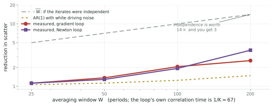
Polyak-Ruppert averaging

Average the iterates. Attains the optimal asymptotic covariance with no curvature estimate anywhere.

Zap stochastic approximation

Estimate the Jacobian on a fast timescale, invert it, use it as a matrix gain. A stochastic Newton-Raphson method.

If the goal is terminal variance, averaging already wins. This deck asks the other question: what does a matrix gain buy on a wind turbine, and can we even build one?

The honest framing is that Zap is not the cheapest route to low variance. What it offers is transient behaviour, stability under weak conditions, and conditioning in more than one dimension. Those are the goods worth chasing here, and they happen to line up with the complaint Rotea actually made, which was about tuning effort rather than about noise.

Zap in four lines

\[ \begin{aligned} \hat A_{n+1} &= \hat A_n + \varepsilon_{n+1}\big[A_{n+1} - \hat A_n\big] \\[0.15em] \theta_{n+1} &= \theta_n + \alpha_{n+1}\, G_{n+1}\, f_{n+1}(\theta_n) \\[0.15em] A_{n+1} &= \partial_\theta f_{n+1}(\theta_n) \\[0.15em] G_{n+1} &= -\big[\varepsilon I + \hat A^{\!\top}_{n+1}\hat A_{n+1}\big]^{-1}\hat A_{n+1} \end{aligned} \]

with the two step sizes satisfying \(\varepsilon_n/\alpha_n \to \infty\).

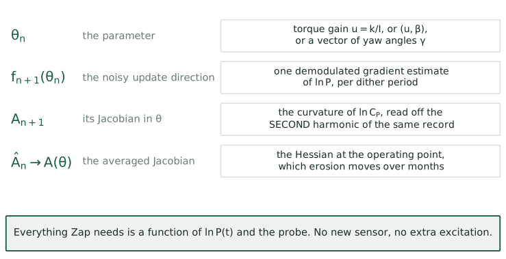
Line three is the whole problem. A is the Jacobian of the sample update direction, differentiated in the parameter. In Q-learning \(f_{n+1}\) is piecewise linear in \(\theta\), so that derivative is free and rank one. A demodulated gradient estimate has no such closed form.

The dictionary

Read the third row twice. It is the claim that makes the rest of the deck possible, and the next three slides are its derivation.

What \(f\) is, precisely

The objective is the turbulence-averaged log-power, \(\Gamma(\theta) = \mathbb{E}\big[\ln P(\theta)\big]\), and because \(3\ln V\) does not depend on \(\theta\) this equals \(\mathbb{E}[\ln C_P]\) up to a constant.

The mean field is \(\bar f(\theta) = \nabla\Gamma(\theta)\). The sample is one dither period of demodulation:

\[f_{n+1}(\theta_n) \;=\; \hat g_n \;=\; \frac{2}{aT}\int_{nT}^{(n+1)T}\ln P(t)\,\sin\omega t\;dt\]

So \(f\) is exactly what LP-ESC already computes. Nothing changes in the forward path. Zap only changes what multiplies \(\hat g_n\) before it reaches the integrator.

What \(A\) is, precisely

\[A(\theta) \;=\; \partial_\theta \bar f(\theta) \;=\; \nabla^2\Gamma(\theta)\]

For the torque-gain problem this is the scalar \(\partial^2 \ln C_P/\partial u^2\) at the operating point. It is the same number that appears in Rotea’s 2017 crossover frequency,

\[\nu_c \;=\; \frac{\kappa}{C_P^{\max}}\left|\frac{\partial^2 C_P}{\partial u^2}(u_o)\right|\]

The curvature is not a new quantity being introduced. It is already in the tuning formula, taken on faith from a design curve. Zap proposes to measure it instead.

Where \(A_{n+1}\) comes from

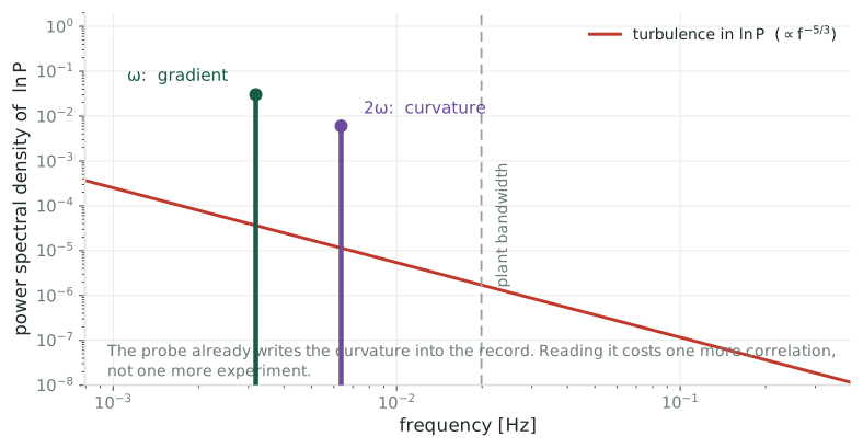
The probe already writes the curvature into the data. Nobody reads it.

Expand around the operating point

Put \(\theta(t) = \theta_n + a\sin\omega t\) into a local quadratic model of \(y = \ln P\), with \(g\) the slope and \(H\) the curvature at \(\theta_n\):

\[y(t) \;=\; \text{const} \;+\; g\,a\sin\omega t \;+\; \tfrac12 H a^2 \sin^2\!\omega t\]

Now use \(\sin^2\omega t = \tfrac12(1 - \cos 2\omega t)\):

\[y(t) \;=\; \underbrace{\Big[\,\cdot\, + \tfrac14 H a^2\Big]}_{\text{DC}} \;+\; \underbrace{g\,a\,\sin\omega t}_{\text{first harmonic}} \;-\; \underbrace{\tfrac14 H a^2\cos 2\omega t}_{\text{second harmonic}}\]

The gradient sits at \(\omega\). The curvature sits at \(2\omega\). They are in the same record, separated in frequency, and one probe generates both.

In the spectrum

Two things to note on this picture. The curvature line is smaller than the gradient line by roughly a over four times the distance from the peak, so close to the optimum it is the larger of the two. And because turbulence falls off as f to the minus five thirds, the noise floor under the second harmonic is about three times lower in power than under the first.

The two demodulators

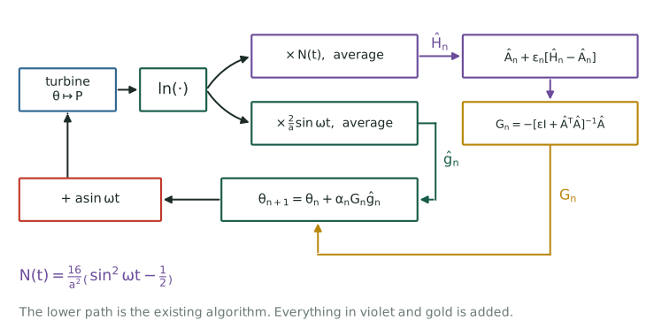
\[ \hat g_n \;=\; \Big\langle\, y\cdot \tfrac{2}{a}\sin\omega t \,\Big\rangle, \qquad \hat H_n \;=\; \big\langle\, y \cdot N(t) \,\big\rangle, \qquad N(t) = \frac{16}{a^2}\left(\sin^2\!\omega t - \frac12\right) \]

Check the second one: \(N(t) = -\tfrac{8}{a^2}\cos 2\omega t\), and averaging it against \(-\tfrac14 H a^2\cos2\omega t\) gives \(\tfrac14 H a^2 \cdot \tfrac{8}{a^2}\cdot\tfrac12 = H\).

\(A_{n+1} = \hat H_n\). One extra correlation against a signal you already generate. No new sensor, no extra excitation, no additional load on the machine.

This demodulation pair is not new. It is the Newton-based extremum seeking of Ghaffari, Krstic and Nesic, Automatica 2012, which also supplies a Riccati filter that converges to the inverse of H without ever inverting a matrix. That paper is not in our literature folder and I am working from memory, so the attribution needs checking before it goes in a proposal.

What is new here is the pairing: their demodulation supplies Zap’s missing Jacobian, and Zap supplies the asymptotic covariance theory and the regularized pseudo-inverse that their Riccati filter lacks.

More than one parameter

For \(\theta \in \mathbb{R}^p\), dither each component at its own frequency and demodulate with a matrix:

\[ N_{ii}(t) = \frac{16}{a_i^2}\left(\sin^2\!\omega_i t - \frac12\right), \qquad N_{ij}(t) = \frac{4}{a_i a_j}\,\sin\omega_i t\,\sin\omega_j t \quad (i\neq j) \]

The frequencies must satisfy the usual separation conditions, and now also \(2\omega_i\) must not collide with any \(\omega_j\) or \(\omega_j \pm \omega_k\). For six yawed turbines that is a real combinatorial constraint on a narrow usable band.

The loop, assembled

The lower path is LP-ESC exactly as published. Everything added is a second correlation and two recursions, all on signals already in hand.

What it buys

Three things, and only one of them is about noise.

The curvature leaves the loop gain

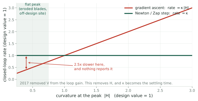
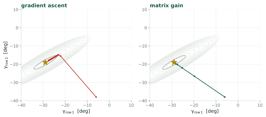
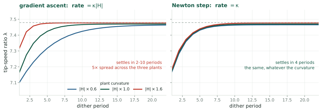
Write \(\delta = \theta - \theta^\star\), so \(g = H\delta\) with \(H<0\) at a maximum. Gradient ascent linearizes to \(\dot\delta = \kappa H\delta\), stable at rate \(\kappa|H|\). Meyn’s gain carries its own sign, \(G = -H/(\varepsilon+H^2)\), and with \(\varepsilon\to 0\) the update gives \(\dot\delta = -\kappa\delta\).

2017 removed \(V\) from the loop gain. This removes \(H\). What is left is \(\kappa\), which now is the settling time rather than merely influencing it.

Which is the tuning complaint, answered

What Rotea wrote

A version of ESC that “converges very fast but it takes too long to tune its parameters.”

What the TORQUE paper says

“All parameters with the exception of dither frequency and amplitude were obtained by trial and error.”

Under gradient ascent, \(\kappa\) has to be re-found whenever \(H\) changes, and \(H\) changes with the site, with the blade condition, and with the operating point. Under a matrix gain, \(\kappa\) is set once from the settling time you want.

This is the strongest single argument in the deck, because it addresses the thing he actually complained about rather than the thing the literature is organised around. Note that it holds even in the scalar case, where the matrix gain is just division by an estimated number.

Where a matrix really pays

Gradient methods converge at a rate set by the smallest Hessian eigenvalue. The measured farm power maps in the twelve-turbine tunnel experiment are long narrow ridges in the yaw angles, which is precisely the case where that hurts.

In the scalar torque-gain problem a matrix gain is a convenience. In the yaw problem it is the difference between converging and crawling, because the wake interaction makes the objective strongly anisotropic and there is no reason the principal axes should line up with individual turbines.

Regularization is doing real work

In the scalar case \(G = -\hat A/(\varepsilon + \hat A^2)\), so the effective rate is

\[\kappa\,\frac{H^2}{\varepsilon + H^2}\]

On a flat peak \(\hat A \to 0\) and an unregularized Newton step would explode. This form does the opposite: it backs off to a small step, degrading gracefully into gradient ascent exactly where curvature cannot be seen.

Worth stressing because the C_P peak is flat by design and gets flatter as the blades degrade. A naive inverse-Hessian method on this plant would be dangerous. The epsilon in Meyn’s formula is not a numerical detail here, it is the safety property that makes the method usable.

What it costs

Three objections. One of them is a hard gate.

The curvature estimate is noisier, but not where it matters

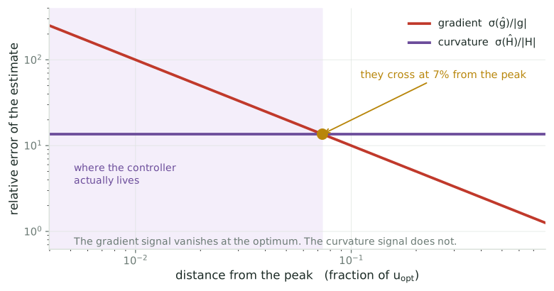
In absolute terms \(\sigma(\hat H)/\sigma(\hat g) \approx (8/a)\,2^{-5/6} \approx 14\) at the published dither amplitude.

But the gradient signal vanishes at the optimum and the curvature signal does not. In relative terms the two cross at about 7% of \(u_{opt}\) from the peak, and inside that the curvature is the better conditioned of the two.

This is the result I did not expect. The received wisdom is that second-order information is hopeless under noise, and in absolute terms that is right. But a controller near convergence is estimating a gradient whose true value is approaching zero, so its relative error diverges, while the curvature it is trying to measure stays put. The regime where Newton methods are supposed to be impossible is the regime where the turbine actually operates.

The gate: \(2\omega\) must fit inside the plant

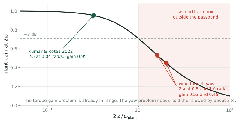
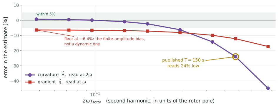
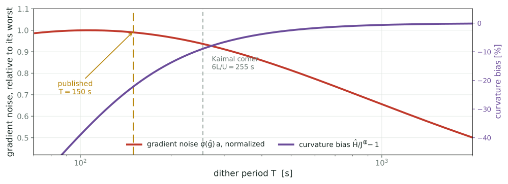
The rotor is a low-pass filter. If \(2\omega\) falls outside its passband the second harmonic is attenuated and phase-shifted, and the curvature estimate is biased by an amount nobody is tracking.

The numbers decide feasibility case by case. For the torque-gain problem in Kumar and Rotea 2022, the plant time constant is 8 seconds and the dither is 0.02 radians per second, so two omega lands at 0.32 of the bandwidth: gain 0.95, phase lag 18 degrees. That is comfortably usable.

For the wind tunnel yaw work the plant time constant is 2 seconds and the dither is 0.4 to 0.5 radians per second, so two omega lands at 1.6 to 2.0 times the bandwidth: gain 0.45 to 0.53, phase lag close to 60 degrees. Not usable as tuned. The dither would have to be slowed by roughly a factor of three, which costs convergence time and partly undoes the reason LP-PIESC was attractive there.

This also sharpens the earlier observation about dither frequencies creeping upward across this line of work. Reading the second harmonic halves the usable dither band.

The timescales are the wrong way round

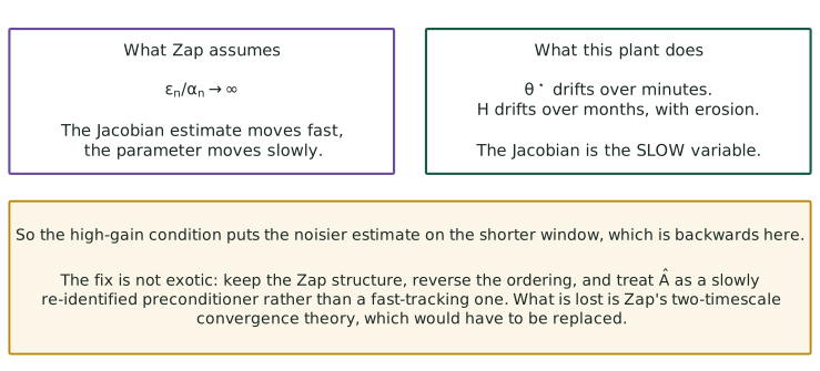
Zap’s high-gain condition \(\varepsilon_n/\alpha_n \to \infty\) puts the noisier estimate on the shorter averaging window. That is right when the Jacobian is cheap, as in Q-learning. It is backwards here.

The curvature of the C_P surface is a property of the blade. It changes as the blade erodes, over weeks and months. The optimum itself moves faster than that, with the operating point. So the natural design is the reverse of Zap: identify A slowly and carefully, and let theta move on the faster timescale.

That is a defensible algorithm, but it is no longer Zap, and Meyn’s two-timescale convergence theory does not cover it. Something would have to be put in its place. This is the part of the proposal that is genuinely open rather than merely unimplemented.

Zap against averaging

What averaging gives you

The optimal asymptotic covariance. Free. No Jacobian, no second demodulator, no frequency budget, no bandwidth constraint.

What the matrix gain adds

Gain calibration, transient behaviour, and conditioning in more than one dimension. It does not improve the terminal variance.

So the case for Zap here has to rest on tuning effort and on the multivariable yaw problem. If it is argued on variance it will lose to four lines of averaging.

Without extremum seeking

Drop the demodulation apparatus and run stochastic approximation directly.

What is left when ESC goes

What gets deleted

The dither frequency, the phase compensation \(\theta\), the high-pass and low-pass filters, the lock-in multiplier, the requirement that \(2\omega\) fit inside the plant passband.

What is left

\[\theta_{n+1} = \theta_n + \alpha_n\,G_n\,\hat g_n\]

Perturb, hold, measure, update. The SA recursion with nothing wrapped around it.

An iteration is now a small number of held operating points, each averaged long enough to see through the turbulence, rather than a continuous sinusoid the machine rides.

This is a different algorithm, not extremum seeking with the tone replaced by noise. Worth being clear about, because the objection from the QSA literature is aimed at the second thing and does not transfer cleanly to the first.

The gradient: SPSA

Draw \(\Delta_n\) with independent \(\pm1\) entries, perturb every parameter at once, and take one difference:

\[\hat g_n \;=\; \frac{\bar y(\theta_n + c\Delta_n) - \bar y(\theta_n - c\Delta_n)}{2c} \begin{bmatrix}\Delta_{n1}^{-1}\\ \vdots \\ \Delta_{np}^{-1}\end{bmatrix}\]

where \(\bar y\) is the mean of \(\ln P\) over a held window.

Two measurements, whatever \(p\) is. That is the property the deterministic scheme cannot match, and it is the entire case for going stochastic on this plant.

Where \(A_{n+1}\) comes from now

The second harmonic is gone with the tone. Two replacements:

Spall’s 2SPSA

A second perturbation \(\tilde\Delta_n\), two more gradient estimates, and a symmetrized outer product

\[\hat H_n = \tfrac12\Big[\tfrac{\delta \hat g_n}{2\tilde c}\tilde\Delta_n^{-\top} + (\cdot)^{\!\top}\Big]\]

Rank two per iteration, four measurements.

Gaussian probe and Stein

For \(\xi \sim N(0,I)\), the second-order Stein identity gives

\[\mathbb{E}\big[\,y\,(\xi\xi^{\!\top} - I)\,\big] = a^2\,\nabla^2\Gamma\]

so \(\hat H_n = \langle y(\xi\xi^{\!\top}-I)\rangle/a^2\). No second perturbation.

Either way \(A_{n+1} = \hat H_n\), the running average is Zap’s (8.51a), and the regularized inverse is unchanged. Spall’s 2SPSA is Zap with SPSA supplying the Jacobian.

The 2SPSA measurement count needs checking against Spall’s 2000 TAC paper, which is not in our folder. I have it as four per iteration with reuse, but the accounting varies between presentations.

The Bernoulli trap

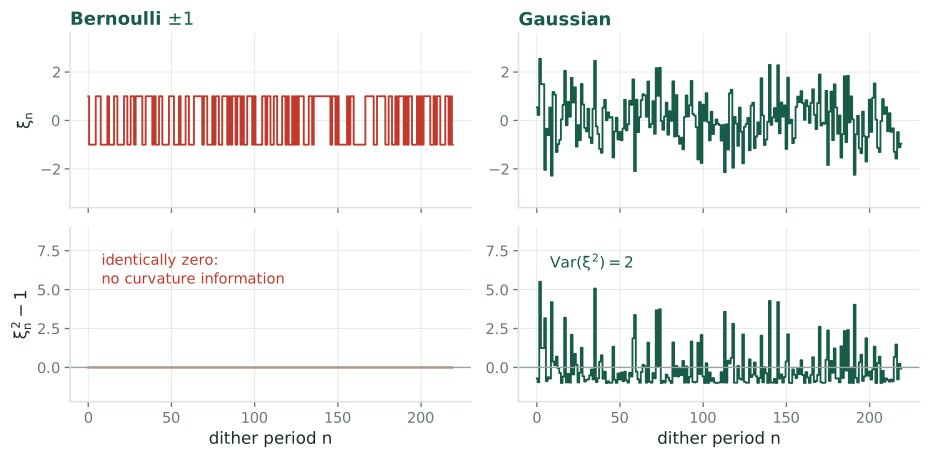
The natural stochastic analogue of the 2019 square wave is a random \(\pm1\) sign sequence. It gives the gradient, but \(\xi^2 \equiv 1\), so \(\mathrm{Var}(\xi^2)=0\) and the Stein estimator divides by zero. Bernoulli probing carries no curvature information at all.

Verified numerically: with a plus-minus-one probe, g-hat recovers the true gradient to four decimals while the curvature estimate is undefined. With a Gaussian probe of the same amplitude, both come back correct.

So the choice of perturbation distribution is not cosmetic. If you want the Hessian for one extra correlation rather than four extra measurements, the probe must have a non-degenerate fourth moment.

What it costs

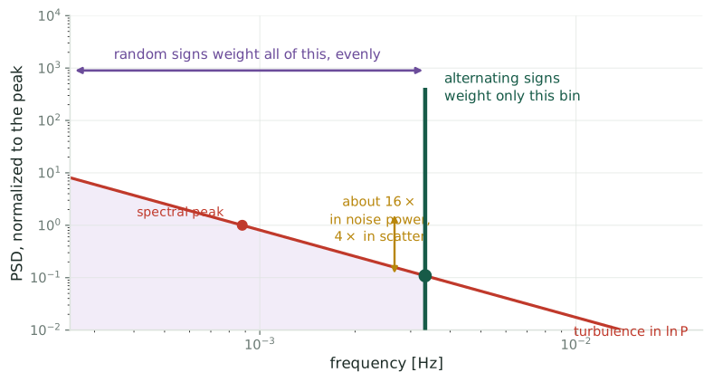
Both schemes difference two windows, so both reject DC. The difference is where each weights the turbulence.

An alternating sign sequence concentrates the estimator’s noise weighting in one bin, which you place above the spectral peak. A random sequence is white, so it weights everything below its Nyquist frequency evenly, including the energy-containing range. Roughly \(16\times\) in noise power, \(4\times\) in the scatter of \(\hat g\).

There is a second cost that does not show on this plot. ESC dithers continuously and treats the rotor response as part of a transfer function, with phase compensation absorbing the lag. Holding a perturbed operating point means waiting out the rotor, about six seconds of time constant, so roughly thirty seconds of dead time before the averaging window can even start. At four to six measurements per iteration that is two to three minutes of the budget spent settling rather than measuring.

What it buys

The deterministic Hessian needs a separate channel for every entry of \(\nabla^2\Gamma\), at a distinct frequency product, none colliding with any \(\omega_k\) or \(2\omega_k\), all inside the plant bandwidth.

parameters \(p\)	frequency slots needed	2SPSA measurements
1, torque gain	2	4
2, torque and pitch	6	4
6, yaw, optimized jointly	58	4

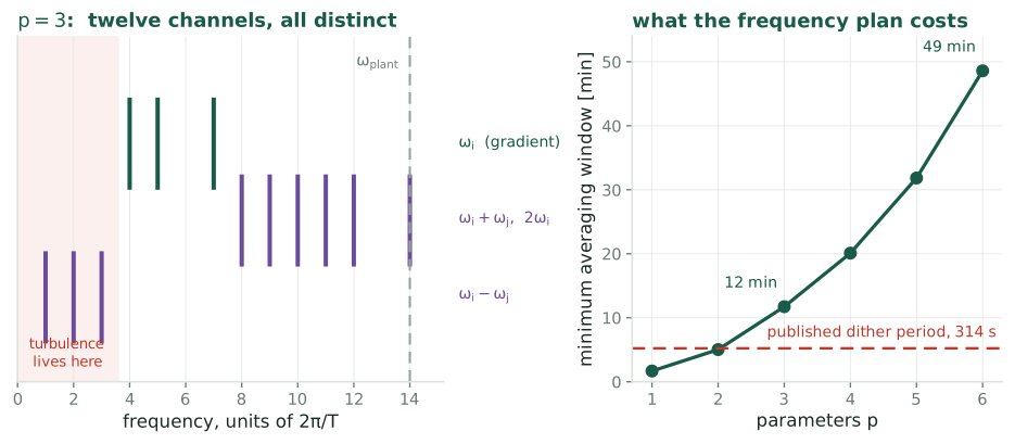
At \(p=1\) the tone wins on every axis. At \(p=6\) the plan needs 58 slots, so the averaging window has to stretch to 49 minutes before noise is even considered, and the stochastic version becomes the only one that runs.

The two Hessians, compared

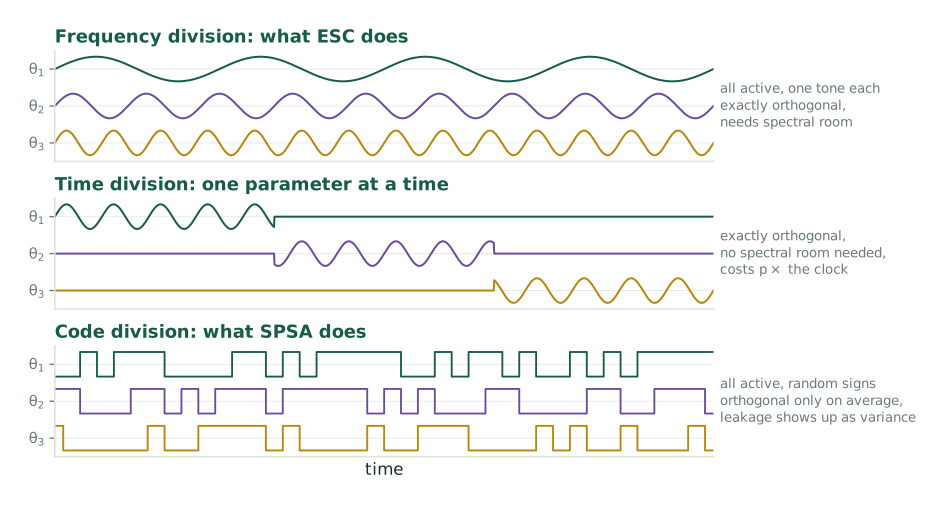
Same matrix, two ways of measuring it, and the difference is combinatorial.

Why frequencies at all

There is one measurement, \(\ln P(t)\), and \(p\) unknowns. The dither frequencies are a multiplexing scheme, nothing more. Distinct \(\omega_i\) make the demodulation channels orthogonal, since \(\langle \sin\omega_i t\,\sin\omega_j t\rangle = \tfrac12\delta_{ij}\).

Share a frequency between two parameters and the cross term stops vanishing, so you read back the sum of two gradient components with no way to split them. Same tone means same channel.

Seen this way the whole tone-versus-random question is a choice of multiplexing. Frequency division is exactly orthogonal but needs spectral room. Code division needs none, but random codes are orthogonal only in expectation, so the leakage between parameters survives in any finite sample and appears as variance. That leakage is the extra scatter we costed out two slides ago.

What the Hessian costs in frequency

The quadratic term produces products, and \(\sin\omega_i t \sin\omega_j t = \tfrac12[\cos(\omega_i-\omega_j)t - \cos(\omega_i+\omega_j)t]\). So \(H_{ij}\) appears at sum and difference frequencies and \(H_{ii}\) at \(2\omega_i\). Every member of

\[\{\omega_k\} \;\cup\; \{2\omega_k\} \;\cup\; \{\omega_i \pm \omega_j\}\]

must be distinct, and all of it must fit below \(\omega_{plant}\).

That is stronger than a Sidon set, because the gradient tones must also avoid every second-order product. A plain Golomb ruler is necessary and not sufficient.

And it grows quadratically

\(p\)	a valid tone set	widest product	minimum window
1	\(\{1\}\)	2	101 s
3	\(\{4,5,7\}\)	14	704 s
6	\(\{4,10,17,26,28,29\}\)	58	2915 s

Computed by exhaustive search over the full condition, not from the asymptotic Sidon bound, with the widest product required to sit inside a plant bandwidth of 0.125 radians per second.

Two things to take from the left panel. The band fills from both ends, and the difference frequencies land close to DC, which is exactly where turbulence is strongest. So the off-diagonal Hessian channels are placed in the worst part of the spectrum by the algebra rather than by choice.

And note where 314 seconds sits on the right panel. The published tuning has room for two parameters and no more.

Head to head

	ESC, second harmonic	SA, 2SPSA or Stein
separation	frequency division	code division
orthogonality	exact, over one period	in expectation only
measurements per update	0 extra, same window	4 extra
spectral demand	grows as \(p^2\)	none
noise weighting	one chosen bin	whole band below Nyquist
scatter in \(\hat g\)	reference	about \(4\times\) worse
settling dead time	none, rides continuously	about \(5\tau\) per held point
perturbation seen by the drivetrain	smooth sinusoid	step changes
degenerate cases	tones colliding with products	Bernoulli probe, \(\mathrm{Var}(\xi^2)=0\)

The tone wins every row except one. That row is spectral demand, and it is the row that decides the farm-scale problem.

Reading the table honestly

\(p \le 2\)

The frequency plan is trivial and the tone is better on every axis that matters. There is no argument for random probing here.

\(p \ge 4\)

The plan needs a 20 to 50 minute window before noise even enters. Random probing is not merely competitive, it is the only scheme that runs.

The load row deserves more weight than it usually gets. Kumar and Rotea 2022, Figure 13: the single step in torque gain when the controller switches on raises drivetrain torsion DEL by 70% at 4 m/s. SPSA makes a step like that every iteration, in both directions, and nobody has costed that out.

The synthesis this points to

Both columns assume the Hessian must be measured at the same rate as the gradient. Nothing in the problem requires that.

Gradient

Keep the tone. Continuous, gentle, low-noise, and only \(p\) frequencies are needed when no products have to be resolved.

Curvature

A deliberate experiment, run rarely. \(H\) drifts with erosion, over months. Once a week is often enough.

In between

Use the last estimate as a slowly refreshed preconditioner, which is Zap with the timescales put the right way round.

Run rarely, the curvature experiment can be time-division multiplexed: sweep one parameter at a time. No frequency plan, no \(2\omega\) constraint, no \(p^2\) bandwidth, and no random probing either.

This is the answer the two halves of the deck converge on. The whole tone-against-noise argument is a fight over how to squeeze p-squared channels through a narrow band every single iteration, and the premise of that fight is wrong. The gradient needs to be fast because it is chasing a moving optimum. The curvature does not, because it is tracking blade wear.

Separate the two rates and the combinatorial problem dissolves, because sequential excitation is admissible once you are not in a hurry.

Verdict

Tone, feasible now

Single-turbine torque gain. \(2\omega\) sits at 0.32 of the plant bandwidth at the published tuning, and with \(p=1\) there is no frequency plan to solve.

Tone, after retuning

Two parameters, \((u,\beta)\). Three demodulation channels to place, and the bandwidth is there for them.

Random probing

Yaw across a farm, optimized jointly. This is not what the tunnel experiment does: it runs six scalar loops on clusters, which is how it keeps \(p=1\).

Both versions share everything downstream of the Jacobian: the averaging recursion, the regularized inverse, the Polyak-Ruppert tail. Only the way \(A_{n+1}\) is measured changes, so the two are the same program with two front ends.

What I would test first

P0, two weeks

Run the existing LP-ESC at a fixed torque gain, demodulate at \(2\omega\), and compare \(\hat H\) against the curvature of the simulator’s own \(C_P\) surface. Pure measurement, no loop closed.

The gate

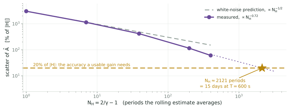
Does \(\hat H\) converge to within, say, 20% over a plausible averaging window, and does its scatter match the \((8/a)2^{-5/6}\) prediction?

If \(\hat H\) can be measured open-loop, everything else in this deck is engineering. If it cannot, the matrix gain is dead and Polyak-Ruppert averaging is the whole answer to Rotea’s question.

Note what this test does not require: closing the loop, retuning anything, or committing to Zap. It asks only whether the second harmonic carries usable curvature on this plant, which is the single fact everything else depends on.

A matrix gain for extremum seeking

The Jacobian Zap needs is measurable: one octave up from the gradient, or in the second moment of a random probe.

The mapping

\(f\) is a gradient estimate, from a tone or from a random perturbation. \(A\) is the curvature of \(\ln C_P\), read at \(2\omega\) or from a second moment. \(\hat A\) is the Hessian that erosion moves.

The open part

Which front end to use is set by \(p\), not by taste. Still open: a convergence theory for the reversed timescale ordering this plant actually wants.

Meyn, Control Systems and Reinforcement Learning, §8.5 · Ghaffari, Krstic & Nesic, Automatica 2012 · Spall, IEEE TAC 2000 (both attributions to be checked) · Kumar & Rotea, Energies 2022 · Rotea et al., TORQUE 2024

Companion to Climbing a Hill You Cannot See.