Inverted Pendulum, Magnetic Levitation, and Cart on a Track

System Modeling and Control · Chapter 13

John N. Chiasson and Aykut C. Satici

Contents

• Inverted-Pendulum Modeling

• Linearization About Equilibrium Points

• Magnetic-Levitation Modeling

• Linear and Transfer-Function Models

• Cart-on-a-Track Modeling

Inverted Pendulum

Control Objective

• Keep the pendulum rod upright (vertical so that \(\theta =0\)).

• The input force \(u(t)\) is to be used to keep \(\theta =0.\)

• In this chapter we derive the mathematical model of the inverted pendulum.

• Control of the pendulum is considered using nested PD controllers.

Mathematical Model of the Inverted Pendulum

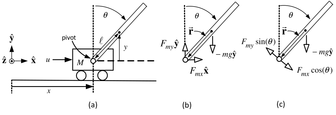
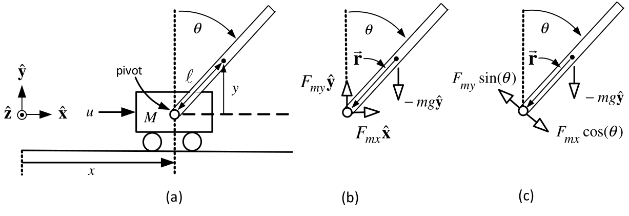
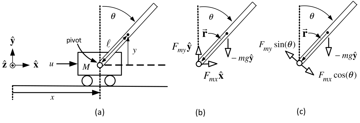
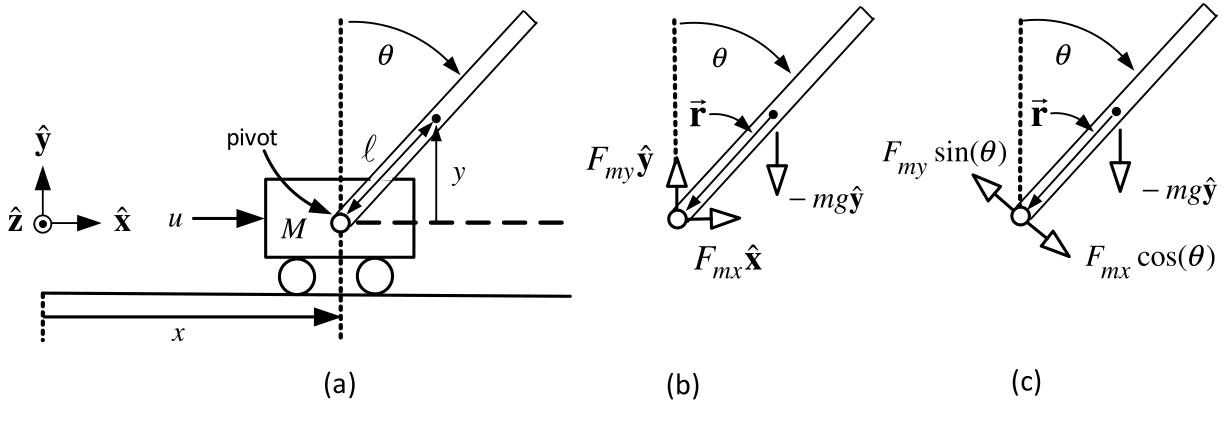
• \(u(t)\) is the force on the cart in the horizontal direction.

• The center of mass (CoM) of the pendulum rod is at \((x+\ell \sin (\theta ),y).\)

• The pendulum rod of length \(2\ell\) is free to rotate about the pivot.

• \(M\) is the cart’s mass and \(m\) is the mass of the pendulum rod.

• There is a sensor to measure the angle \(\theta\) between the rod and the vertical.

Mathematical Model of the Inverted Pendulum

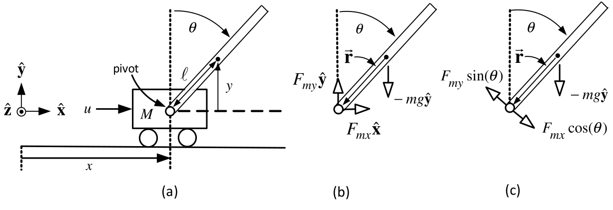
• The pivot exerts a force \(\boldsymbol{F}_{m}\) on \(m\) through the rod. \[\boldsymbol{F}_{m}=F_{mx}\mathbf{\hat{x}}+F_{my}\mathbf{\hat{y}}\]

• \(-\boldsymbol{F}_{m}=-F_{mx}\mathbf{\hat{x}}-F_{my}\mathbf{\hat{y}}\) is the reaction force of the rod on the cart.

• The center of mass (CoM) of the pendulum rod is at \((x+\ell \sin (\theta ),y).\)

• The axis of rotation for the rod is in the \(-\mathbf{\hat{z}}\) direction through its CoM.

Mathematical Model of the Inverted Pendulum

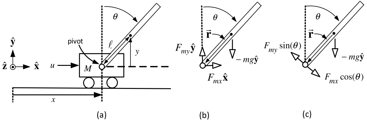
Equations of linear motion for \(m\): \[\begin{aligned} m\frac{d^{2}}{dt^{2}}\left( x+\ell \sin (\theta )\right) &=F_{mx} \\ m\frac{d^{2}}{dt^{2}}\left( \ell \cos (\theta )\right) &=F_{my}-mg \end{aligned}\]

Mathematical Model of the Inverted Pendulum

• The axis of rotation for the rod is in the \(-\mathbf{\hat{z}}\) direction through its CoM.

• If your right thumb is pointing in the \(-\mathbf{\hat{z}}\) direction, then your fingers

  are pointing in the positive \(\theta\) direction.

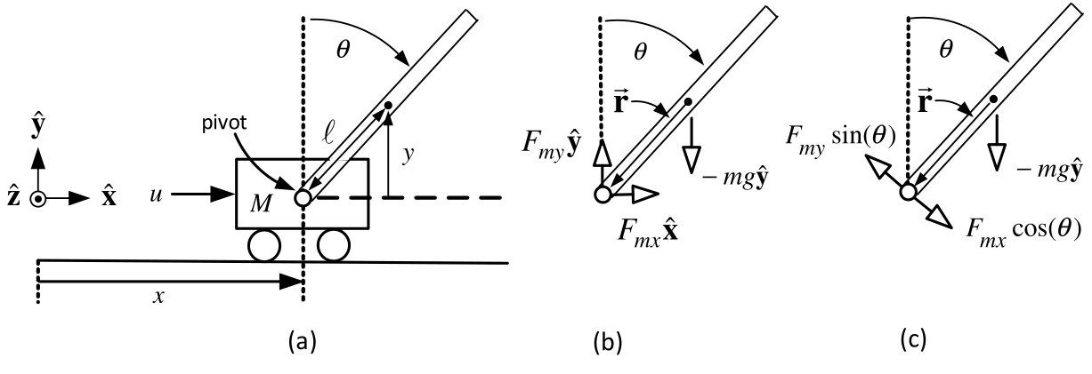
• \(J=m\ell ^{2}/3\) is the moment of inertia of rod with respect to its axis of rotation.

• The rod is accelerating, but \[\tau =J\dfrac{d^{2}\theta }{dt^{2}}\] is still valid as the rotation axis is through the CoM.

Mathematical Model of the Inverted Pendulum

• The gravitational force \(-mg\mathbf{\hat{y}}\) does not produce any torque on the rod\(.\)

  • It acts through the center of mass so its moment arm zero.

• The force \(F_{my}\mathbf{\hat{y}}\) has the component \(F_{my}\sin (\theta )\) perpendicular to the rod.

• The force \(F_{mx}\mathbf{\hat{x}}\) has the component \(F_{mx}\cos (\theta )\) perpendicular to the rod. \(.\)

Eqn of rotational motion: \(\ J\dfrac{d^{2}\theta }{dt^{2}}=\ell F_{my}\sin (\theta )-\ell F_{mx}\cos (\theta ).\)

Eqn of motion of the cart: \(\ M\dfrac{d^{2}x}{dt^{2}}=u(t)-F_{mx}.\)

Mathematical Model of the Inverted Pendulum

Complete set of equations of motion: \[\begin{aligned} m\frac{d^{2}}{dt^{2}}\left( x+\ell \sin (\theta )\right) &=F_{mx} \\ m\frac{d^{2}}{dt^{2}}\left( \ell \cos (\theta )\right) &=F_{my}-mg \\ J\frac{d^{2}\theta }{dt^{2}} &=\ell F_{my}\sin (\theta )-\ell F_{mx}\cos (\theta ) \\ M\frac{d^{2}x}{dt^{2}} &=u(t)-F_{mx}. \end{aligned}\]

Mathematical Model of the Inverted Pendulum

\[\begin{aligned} m\frac{d^{2}}{dt^{2}}\left( x+\ell \sin (\theta )\right) &=F_{mx} \\ m\frac{d^{2}}{dt^{2}}\left( \ell \cos (\theta )\right) &=F_{my}-mg \\ J\frac{d^{2}\theta }{dt^{2}} &=\ell F_{my}\sin (\theta )-\ell F_{mx}\cos (\theta ) \\ M\frac{d^{2}x}{dt^{2}} &=u(t)-F_{mx}. \end{aligned}\] Expand: \[\begin{aligned} m\frac{d^{2}x}{dt^{2}}-m\ell \sin (\theta )\left( \frac{d\theta }{dt} \right) ^{2}+m\ell \cos (\theta )\frac{d^{2}\theta }{dt^{2}} &=F_{mx} \\ -m\ell \cos (\theta )\left( \frac{d\theta }{dt}\right) ^{2}-m\ell \sin (\theta )\frac{d^{2}\theta }{dt^{2}} &=F_{my}-mg \\ \ell F_{my}\sin (\theta )-\ell F_{mx}\cos (\theta ) &=J\frac{d^{2}\theta }{ dt^{2}} \\ u(t)-F_{mx} &=M\frac{d^{2}x}{dt^{2}}. \end{aligned}\]

Mathematical Model of the Inverted Pendulum

\[\begin{aligned} m\frac{d^{2}x}{dt^{2}}-m\ell \sin (\theta )\left( \frac{d\theta }{dt} \right) ^{2}+m\ell \cos (\theta )\frac{d^{2}\theta }{dt^{2}} &=F_{mx} \\ -m\ell \cos (\theta )\left( \frac{d\theta }{dt}\right) ^{2}-m\ell \sin (\theta )\frac{d^{2}\theta }{dt^{2}} &=F_{my}-mg \\ \ell F_{my}\sin (\theta )-\ell F_{mx}\cos (\theta ) &=J\frac{d^{2}\theta }{ dt^{2}} \\ u(t)-F_{mx} &=M\frac{d^{2}x}{dt^{2}}. \end{aligned}\]

Eliminate the reaction forces \(F_{mx},F_{my}\). \[\begin{aligned} mg\ell \sin (\theta )-m\ell \cos (\theta )\frac{d^{2}x}{dt^{2}} &=(J+m\ell ^{2})\frac{d^{2}\theta }{dt^{2}} \\ (M+m)\frac{d^{2}x}{dt^{2}}+m\ell \cos (\theta )\frac{d^{2}\theta }{dt^{2}} -m\ell \omega ^{2}\sin (\theta ) &=u(t). \\ \end{aligned}\] Or \[\left[ \begin{array}{cc} J+m\ell ^{2} & m\ell \cos (\theta ) \\ m\ell \cos (\theta ) & M+m \end{array} \right] \left[ \begin{array}{c} d^{2}\theta /dt^{2} \\ d^{2}x/dt^{2} \end{array} \right] =\left[ \begin{array}{c} mg\ell \sin (\theta ) \\ m\ell \omega ^{2}\sin (\theta )+u(t) \end{array} \right] .\]

Mathematical Model of the Inverted Pendulum

Define \[\begin{aligned} H(\theta)&\triangleq \begin{bmatrix} J+m\ell^2 & m\ell\cos\theta\\ m\ell\cos\theta & M+m \end{bmatrix},\\ D(\theta)&\triangleq\det H(\theta) =JM+Jm+Mm\ell^2+m^2\ell^2\sin^2\theta. \end{aligned}\]

The acceleration vector is \[\begin{aligned} \begin{bmatrix}\ddot\theta\\\ddot x\end{bmatrix} &=H(\theta)^{-1} \begin{bmatrix} mg\ell\sin\theta\\ m\ell\omega^2\sin\theta+u \end{bmatrix}\\[0.4em] &=\frac{1}{D(\theta)} \left\{ \begin{bmatrix} gm\ell(M+m)\sin\theta-m^2\ell^2\omega^2\cos\theta\sin\theta\\ m\ell(J+m\ell^2)\omega^2\sin\theta-gm^2\ell^2\cos\theta\sin\theta \end{bmatrix} +\begin{bmatrix} -m\ell\cos\theta\\ J+m\ell^2 \end{bmatrix}u \right\}. \end{aligned}\]

Mathematical Model in Statespace Form

\(v\triangleq \dfrac{dx}{dt},\quad \omega =\dot{\theta}=\dfrac{d\theta }{dt}\).

Define \[D(\theta)\triangleq JM+Jm+Mm\ell ^2+m^2\ell ^2\sin^2\theta.\]

Then \[\begin{aligned} \frac{dx}{dt} &=v \\ \frac{dv}{dt} &=\frac{m\ell (J+m\ell ^2)\omega^2\sin\theta -gm^2\ell^2\cos\theta\sin\theta}{D(\theta)} +\frac{J+m\ell^2}{D(\theta)}u \\ \frac{d\theta }{dt} &=\omega \\ \frac{d\omega }{dt} &=\frac{gm\ell (M+m)\sin\theta -m^2\ell^2\omega^2\cos\theta\sin\theta}{D(\theta)} -\frac{m\ell\cos\theta}{D(\theta)}u. \end{aligned}\]

Mathematical Model in Statespace Form

• The state \(z\) is simply the vector \[z\triangleq \left[ \begin{array}{c} x \\ v \\ \theta \\ \omega \end{array} \right]\]

• \(x,v,\theta ,\) and \(\omega\) are called the state variables .

Statespace Form

• The left-hand side contains only a first-order derivative.

• The right-hand side of each eqn has only state variables and no derivatives.

Linear Approximate Model of the Inverted Pendulum

• The statespace model is nonlinear for which a control design is not known.

• We simplify the model in order to be able to design a controller.

• The objective is to keep the pendulum upright, i.e., \(\theta \approx 0,\omega =\dot{\theta}\approx 0\).

• Make these approximations in the model by setting \[\begin{aligned} \sin (\theta ) &\approx &\theta \\ \cos (\theta ) &\approx &1 \\ \omega ^{2}\sin (\theta ) &\approx &\omega ^{2}\theta \approx 0 \\ \cos \theta \sin \theta &\approx &1\cdot \theta =\theta \\ \sin ^{2}(\theta ) &\approx &\theta ^{2}\approx 0 \\ \omega ^{2}\cos \theta \sin \theta &\approx &\omega ^{2}\cdot 1\cdot \theta \approx 0. \end{aligned}\]

• E.g., if \(\omega =0.01\) (small), then \(\omega ^{2}=0.0001\) is very small.

  • So keep terms with just \(\omega ,\) but discard the really small terms \(\omega ^{2}\).

Linear Approximate Model of the Inverted Pendulum

\[\begin{aligned} \frac{dv}{dt} &=\frac{m\ell (J+m\ell ^{2})\omega ^{2}\sin \theta -gm^{2}\ell ^{2}\cos \theta \sin \theta }{JM+Jm+Mm\ell ^{2}+m^{2}\ell ^{2}\sin ^{2}(\theta )}+ \\ &&\frac{J+m\ell ^{2}}{JM+Jm+Mm\ell ^{2}+m^{2}\ell ^{2}\sin ^{2}(\theta )}u \\ \frac{d\omega }{dt} &=\frac{gm\ell (M+m)\sin \theta -m^{2}\ell ^{2}\omega ^{2}\cos \theta \sin \theta }{JM+Jm+Mm\ell ^{2}+m^{2}\ell ^{2}\sin ^{2}(\theta )}- \\ &&\frac{m\ell \cos \theta }{JM+Jm+Mm\ell ^{2}+m^{2}\ell ^{2}\sin ^{2}(\theta )}u. \end{aligned}\]

Use the above approximations to obtain: \[\begin{aligned} \frac{dv}{dt} &=\frac{-gm^{2}\ell ^{2}}{JM+Jm+Mm\ell ^{2}}\theta +\frac{ J+m\ell ^{2}}{JM+Jm+Mm\ell ^{2}}u \\ \frac{d\omega }{dt} &=\frac{gm\ell (M+m)}{JM+Jm+Mm\ell ^{2}}\theta -\frac{ m\ell }{JM+Jm+Mm\ell ^{2}}u. \end{aligned}\]

Linear Approximate Model of the Inverted Pendulum

\[\begin{aligned} \frac{dx}{dt} &=v \\ \frac{dv}{dt} &=-\frac{gm^{2}\ell ^{2}}{JM+Jm+Mm\ell ^{2}}\theta +\frac{ J+m\ell ^{2}}{JM+Jm+Mm\ell ^{2}}u \\ \frac{d\theta }{dt} &=\omega \\ \frac{d\omega }{dt} &=\frac{mg\ell (M+m)}{JM+Jm+Mm\ell ^{2}}\theta -\frac{ m\ell }{JM+Jm+Mm\ell ^{2}}u. \end{aligned}\]

In matrix form \[\underset{dz/dt}{\underbrace{\left[ \begin{array}{c} dx/dt \\ dv/dt \\ d\theta /dt \\ d\omega /dt \end{array} \right] }}=\underset{A}{\underbrace{\left[ \begin{array}{cccc} 0 & 1 & 0 & 0 \\ 0 & 0 & -\dfrac{gm^{2}\ell ^{2}}{Mm\ell ^{2}+J(M+m)} & 0 \\ 0 & 0 & 0 & 1 \\ 0 & 0 & \dfrac{mg\ell (M+m)}{Mm\ell ^{2}+J(M+m)} & 0 \end{array} \right] }}\underset{z}{\underbrace{\left[ \begin{array}{c} x \\ v \\ \theta \\ \omega \end{array} \right] }}+\underset{b}{\underbrace{\left[ \begin{array}{c} 0 \\ \dfrac{J+m\ell ^{2}}{Mm\ell ^{2}+J(M+m)} \\ 0 \\ -\dfrac{m\ell }{Mm\ell ^{2}+J(M+m)} \end{array} \right] }}u.\]

Linear Approximate Model of the Inverted Pendulum

\[\underset{dz/dt}{\underbrace{\left[ \begin{array}{c} dx/dt \\ dv/dt \\ d\theta /dt \\ d\omega /dt \end{array} \right] }}=\underset{A}{\underbrace{\left[ \begin{array}{cccc} 0 & 1 & 0 & 0 \\ 0 & 0 & -\dfrac{gm^{2}\ell ^{2}}{Mm\ell ^{2}+J(M+m)} & 0 \\ 0 & 0 & 0 & 1 \\ 0 & 0 & \dfrac{mg\ell (M+m)}{Mm\ell ^{2}+J(M+m)} & 0 \end{array} \right] }}\underset{z}{\underbrace{\left[ \begin{array}{c} x \\ v \\ \theta \\ \omega \end{array} \right] }}+\underset{b}{\underbrace{\left[ \begin{array}{c} 0 \\ \dfrac{J+m\ell ^{2}}{Mm\ell ^{2}+J(M+m)} \\ 0 \\ -\dfrac{m\ell }{Mm\ell ^{2}+J(M+m)} \end{array} \right] }}u.\]

• Standard linear approximate model of the inverted pendulum.

• We show with \(u(t)\) of the form \[u(t)=-k_{1}x(t)-k_{2}v(t)-k_{3}\theta (t)-k_{4}\omega (t)\] \(k_{1},k_{2},k_{3},k_{4}\) can be chosen so that \((x(t),v(t),\theta (t),\omega (t))\) stays close to \((0,0,0,0). \ \Longrightarrow\)  The pendulum stays upright and the cart stays at \(x=0.\)

• The above is called a linear statespace model.

• The adjective “linear” refers to the form \[\frac{dz}{dt}=Az+bu.\] I.e., \(Az\) is linear in \(z\) and \(bu\) is linear in \(u\).

Transfer Function Model of the Inverted Pendulum

Take the Laplace transform of \[\frac{d\omega }{dt}=\frac{d^{2}\theta }{dt^{2}}=\frac{mg\ell (M+m)}{ JM+Jm+Mm\ell ^{2}}\theta -\frac{m\ell }{JM+Jm+Mm\ell ^{2}}u\] to obtain \[s^{2}\theta (s)-s\theta (0)-\dot{\theta}(0)=\underset{\alpha ^{2}}{ \underbrace{\dfrac{mg\ell (M+m)}{Mm\ell ^{2}+J(M+m)}}}\theta (s)-\underset{ \kappa m\ell }{\underbrace{\dfrac{m\ell }{Mm\ell ^{2}+J(M+m)}}}U(s).\] With the definitions \[\alpha ^{2}\triangleq \dfrac{mg\ell (M+m)}{Mm\ell ^{2}+J(M+m)}, \kappa =\frac{1}{Mm\ell ^{2}+J(M+m)}\] we have \[s^{2}\theta (s)-\alpha ^{2}\theta (s)=-\kappa m\ell U(s)+s\theta (0)+\dot{ \theta}(0)\] or \[\theta (s)=\text{}\underset{\text{transfer function}}{\underbrace{-\frac{ \kappa m\ell }{s^{2}-\alpha ^{2}}}}U(s)+\frac{s\theta (0)+\dot{\theta}(0) }{s^{2}-\alpha ^{2}}.\]

• \(\mathcal{L}\{\ddot{\theta}(t)\}=s\mathcal{L}\{\dot{\theta}(t)\}-\dot{\theta}(0)=s\left(s\mathcal{L}\{\theta(t)\}-\theta(0)\right)-\dot{\theta}(0).\)

Transfer Function Model of the Inverted Pendulum

\[\theta (s)=\text{}\underset{\text{transfer function}}{\underbrace{-\frac{ \kappa m\ell }{s^{2}-\alpha ^{2}}}}U(s)+\frac{s\theta (0)+\dot{\theta}(0) }{s^{2}-\alpha ^{2}}.\]

• Open-loop poles at \(s=-\alpha <0,\alpha >0.\)

• Open-loop system is unstable.

Transfer Function Model of the Inverted Pendulum

From the statespace model \[\frac{dv}{dt}=\frac{d^{2}x}{dt^{2}}=-\frac{mgm\ell ^{2}}{Mm\ell ^{2}+J(M+m)} \theta +\dfrac{J+m\ell ^{2}}{Mm\ell ^{2}+J(M+m)}u.\] Laplace transform: \[s^{2}X(s)-sx(0)-\dot{x}(0)=-\kappa mgm\ell ^{2}\theta (s)+\kappa (J+m\ell ^{2})U(s)\] or \[\begin{aligned} X(s) &=-\kappa mgm\ell ^{2}\frac{1}{s^{2}} \theta (s)+\kappa (J+m\ell ^{2})\frac{1}{s^{2}}U(s)+\frac{sx(0)+\dot{x}(0)}{ s^{2}} \\ &=-\kappa mgm\ell ^{2}\frac{1}{s^{2}}\left( -\frac{\kappa m\ell }{ s^{2}-\alpha ^{2}}U(s)+\frac{s\theta (0)+\dot{\theta}(0)}{s^{2}-\alpha ^{2}} \right) +\kappa (J+m\ell ^{2})\frac{1}{s^{2}}U(s)+\frac{sx(0)+\dot{x}(0)}{ s^{2}} \\ &=\kappa mgm\ell ^{2}\frac{1}{s^{2}}\frac{\kappa m\ell }{ s^{2}-\alpha ^{2}}U(s)+\kappa (J+m\ell ^{2})\frac{1}{s^{2}} U(s)-\kappa mgm\ell ^{2}\frac{1}{s^{2}}\frac{s\theta (0)+\dot{\theta} (0)}{s^{2}-\alpha ^{2}}+\frac{sx(0)+\dot{x}(0)}{s^{2}} \\ &=\frac{\kappa mgm\ell ^{2}\kappa m\ell +\kappa (J+m\ell ^{2})(s^{2}-\alpha ^{2})}{s^{2}(s^{2}-\alpha ^{2})}U(s)-\kappa mgm\ell ^{2} \frac{1}{s^{2}}\frac{s\theta (0)+\dot{\theta}(0)}{s^{2}-\alpha ^{2}}+\frac{ sx(0)+\dot{x}(0)}{s^{2}} \\ && \end{aligned}\]

Transfer Function Model of the Inverted Pendulum

From previous slide: \[X(s)=\frac{\kappa mgm\ell ^{2}\kappa m\ell +\kappa (J+m\ell ^{2})(s^{2}-\alpha ^{2})}{s^{2}(s^{2}-\alpha ^{2})}U(s)-\kappa mgm\ell ^{2} \frac{1}{s^{2}}\frac{s\theta (0)+\dot{\theta}(0)}{s^{2}-\alpha ^{2}}+\frac{ sx(0)+\dot{x}(0)}{s^{2}}\]

Again using \[\alpha ^{2}\triangleq \dfrac{mg\ell (M+m)}{Mm\ell ^{2}+J(M+m)}, \kappa =\frac{1}{Mm\ell ^{2}+J(M+m)}\]

the expression for \(X(s)\) simplifies to \[X(s)=\underset{G_{X}(s)}{\underbrace{\kappa \frac{\left( J+m\ell ^{2}\right) s^{2}-mg\ell }{s^{2}(s^{2}-\alpha ^{2})}}}U(s)+\frac{p(s,\theta (0),\dot{ \theta}(0),x(0),\dot{x}(0))}{s^{2}(s^{2}-\alpha ^{2})}\] \[\begin{aligned} p(s,\theta (0),\dot{\theta}(0),x(0),\dot{x}(0)) &=x(0)s^{3}+\dot{x} (0)s^{2}+\left( -\kappa mgm\ell ^{2}\theta (0)-\alpha ^{2}x(0)\right) s \\ &\quad-\left( \kappa mgm\ell ^{2}\dot{\theta}(0)+\dot{x}(0)\alpha ^{2}\right) . \end{aligned}\]

• \(G_{X}(s)\) has poles at \(0,0,\alpha ,-\alpha\) and zeros at \(\pm \sqrt{ \dfrac{mg\ell }{J+m\ell ^{2}}}=\pm \sqrt{\dfrac{g}{\ell }}\sqrt{\dfrac{1}{ J/(m\ell ^{2})+1}}.\)

Nested Loop (State Feedback) Controller for the Inverted Pendulum

\[\frac{X(s)}{U(s)}=\frac{\kappa (J+m\ell ^{2})s^{2}-\kappa mg\ell }{ s^{2}(s^{2}-\alpha ^{2})}=\underset{\theta (s)/U(s)}{\underbrace{\frac{ -\kappa m\ell }{s^{2}-\alpha ^{2}}}}\underset{X(s)/\theta (s)}{\underbrace{ \frac{-1}{m\ell }\frac{(J+m\ell ^{2})s^{2}-mg\ell }{s^{2}}}}.\] Nested Loop Control Structure

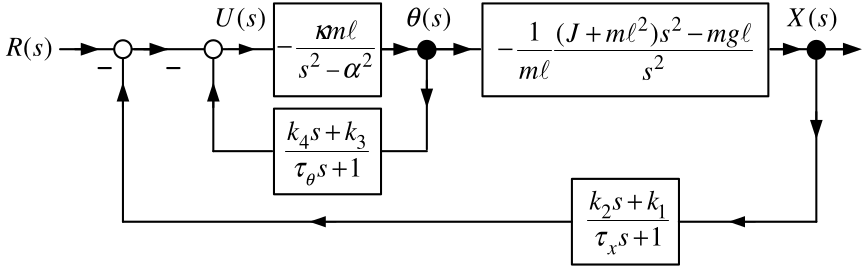
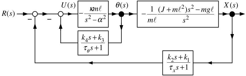
• \(\theta\) and \(x\) are each fed back through a PD controller with low pass filtering.

• The time constants \(\tau _{\theta }\) and \(\tau _{x}\) are small.

• Then \[\begin{aligned} U(s) &=-\frac{k_{1}X(s)+k_{2}sX(s)}{\tau _{x}s+1}-\frac{k_{3}\theta (s)+k_{4}s\theta (s)}{\tau _{\theta }s+1}+R(s) \\ &\approx -k_{1}X(s)-k_{2}sX(s)-k_{3}\theta (s)-k_{4}s\theta (s)+R(s) \end{aligned}\]

• In the time domain (state feedback) \[u(t)\approx -k_{1}x(t)-k_{2}\dot{x}(t)-k_{3}\theta (t)-k_{4}\dot{\theta} (t)+r(t).\]

Nested Loop (State Feedback) Controller for the Inverted Pendulum

Nested Loop Control Structure

Set \(\tau _{\theta }=0,\tau _{x}=0\) as they are small. The Inner loop reduces to \[\frac{-\dfrac{\kappa m\ell }{s^{2}-\alpha ^{2}}}{1-\dfrac{\kappa m\ell }{ s^{2}-\alpha ^{2}}(k_{4}s+k_{3})}=-\frac{\kappa m\ell }{s^{2}-\kappa m\ell k_{4}s-(\alpha ^{2}+\kappa m\ell k_{3})}.\]

Equivalent block diagram

Nested Loop (State Feedback) Controller for the Inverted Pendulum

Closed-loop transfer function \(X(s)/R(s)\)

\[\begin{aligned} \frac{X(s)}{R(s)} &=\frac{\dfrac{\kappa m\ell }{ s^{2}-m\kappa \ell k_{4}s-(\alpha ^{2}+m\kappa \ell k_{3})}\dfrac{1}{m\ell } \dfrac{(J+m\ell ^{2})s^{2}-mg\ell }{s^{2}}}{1+\dfrac{\kappa m\ell }{ s^{2}-m\kappa \ell k_{4}s-(\alpha ^{2}+m\kappa \ell k_{3})}\dfrac{1}{m\ell } \dfrac{(J+m\ell ^{2})s^{2}-mg\ell }{s^{2}}(k_{2}s+k_{1})} \\ &=\frac{\kappa (J+m\ell ^{2})s^{2}-\kappa mg\ell }{ s^{4}-\kappa m\ell k_{4}s^{3}-(\alpha ^{2}+\kappa m\ell k_{3})s^{2}+\kappa ((J+m\ell ^{2})s^{2}-mg\ell )(k_{2}s+k_{1})} \\ &=\frac{\kappa (J+m\ell ^{2})s^{2}-\kappa mg\ell }{ s^{4}+(\kappa k_{2}(m\ell ^{2}+J)-m\kappa \ell k_{4})s^{3}+(\kappa k_{1}(m\ell ^{2}+J)-\alpha ^{2}-m\kappa \ell k_{3})s^{2}-\kappa gm\ell k_{2}s-\kappa gm\ell k_{1}}. \end{aligned}\]

Nested Loop (State Feedback) Controller for the Inverted Pendulum

\[\frac{X(s)}{R(s)}=\frac{\kappa (J+m\ell ^{2})s^{2}-\kappa mg\ell }{s^{4}+(\kappa k_{2}(m\ell ^{2}+J)-m\kappa \ell k_{4})s^{3}+(\kappa k_{1}(m\ell ^{2}+J)-\alpha ^{2}-m\kappa \ell k_{3})s^{2}-\kappa gm\ell k_{2}s-\kappa gm\ell k_{1}}.\]

To obtain the closed-loop characteristic polynomial \(s^{4}+f_{3}s^{3}+f_{2}s^{2}+f_{1}s+f_{0}\) set \[\begin{aligned} f_{3} &=\kappa k_{2}(m\ell ^{2}+J)-\kappa m\ell k_{4} \\ f_{2} &=\kappa k_{1}(m\ell ^{2}+J)-\alpha ^{2}-\kappa m\ell k_{3} \\ f_{1} &=-g\kappa m\ell k_{2} \\ f_{0} &=-g\kappa m\ell k_{1} \end{aligned}\] or \[\left[ \begin{array}{c} f_{3} \\ f_{2} \\ f_{1} \\ f_{0} \end{array} \right] =\left[ \begin{array}{cccc} 0 & \kappa (m\ell ^{2}+J) & 0 & -\kappa m\ell \\ \kappa (m\ell ^{2}+J) & 0 & -\kappa m\ell & 0 \\ 0 & -\kappa mg\ell & 0 & 0 \\ -\kappa mg\ell & 0 & 0 & 0 \end{array} \right] \left[ \begin{array}{c} k_{1} \\ k_{2} \\ k_{3} \\ k_{4} \end{array} \right] +\left[ \begin{array}{c} 0 \\ -\alpha ^{2} \\ 0 \\ 0 \end{array} \right] .\]

Nested Loop (State Feedback) Controller for the Inverted Pendulum

Solve to get \[\left[ \begin{array}{c} k_{1} \\ k_{2} \\ k_{3} \\ k_{4} \end{array} \right] =\left[ \begin{array}{cccc} 0 & \kappa (m\ell ^{2}+J) & 0 & -\kappa m\ell \\ \kappa (m\ell ^{2}+J) & 0 & -\kappa m\ell & 0 \\ 0 & -\kappa mg\ell & 0 & 0 \\ -\kappa mg\ell & 0 & 0 & 0 \end{array} \right] ^{-1}\left[ \begin{array}{c} f_{3} \\ f_{2}+\alpha ^{2} \\ f_{1} \\ f_{0} \end{array} \right] .\] Desired closed-loop poles are \(-r_{1},-r_{2},-r_{3},-r_{4}\), with \(r_i>0\). Set \[\begin{aligned} s^{4}+f_{3}s^{3}+f_{2}s^{2}+f_{1}s+f_{0} &=(s+r_{1})(s+r_{2})(s+r_{3})(s+r_{4}). \end{aligned}\]

Matching coefficients gives \[\begin{aligned} f_{3}&=r_{1}+r_{2}+r_{3}+r_{4},\\ f_{2}&=r_{1}r_{2}+r_{1}r_{3}+r_{1}r_{4} +r_{2}r_{3}+r_{2}r_{4}+r_{3}r_{4},\\ f_{1}&=r_{1}r_{2}r_{3}+r_{1}r_{2}r_{4} +r_{1}r_{3}r_{4}+r_{2}r_{3}r_{4},\\ f_{0}&=r_{1}r_{2}r_{3}r_{4}. \end{aligned}\]

Nested Loop Controller: Tracking Step and Ramp Inputs

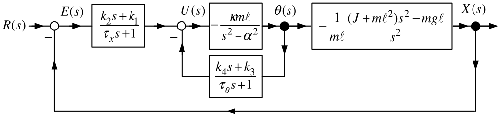
The forward path is type 2.

Not in unity feedback form.

Add the reference input filter \(G_{f}(s)=\dfrac{k_{2}s+k_{1}}{\tau _{x}s+1}.\)

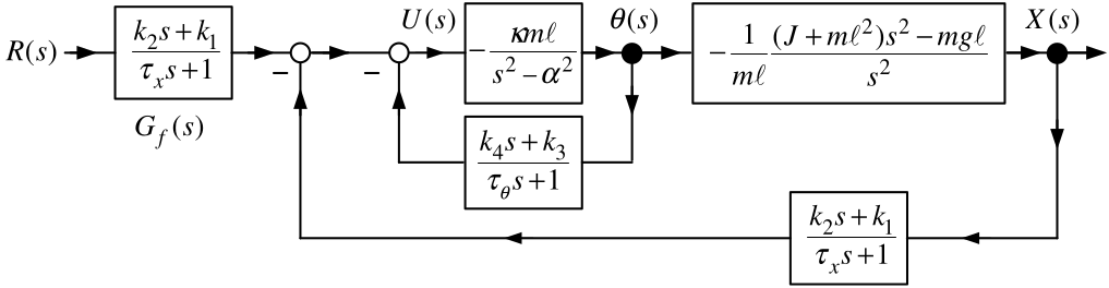
Equivalently it has the unity feedback form.

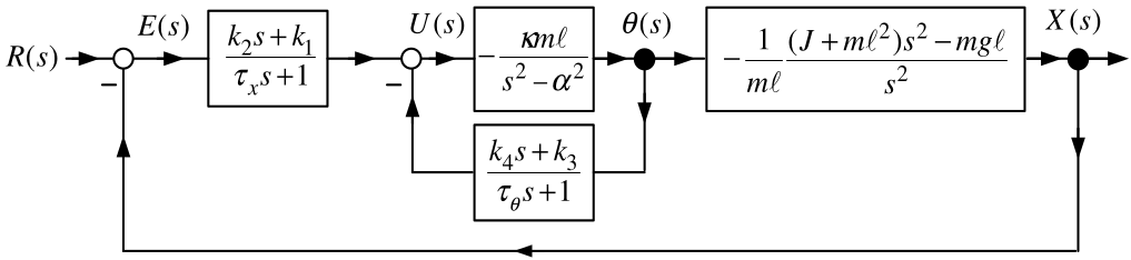
Nested Loop Controller: Tracking Step and Ramp Inputs

Unity feedback form

The error \(E(s)\) is given by \[\begin{aligned} E(s) &=\frac{1}{1+(k_{2}s+k_{1})\dfrac{ \kappa m\ell }{s^{2}-m\kappa \ell k_{4}s-(\alpha ^{2}+m\kappa \ell k_{3})} \dfrac{1}{m\ell }\dfrac{(J+m\ell ^{2})s^{2}-mg\ell }{s^{2}}}R(s) \\ &=\frac{(s^{2}-m\kappa \ell k_{4}s-\alpha ^{2}-m\kappa \ell k_{3})s^{2}}{s^{4}+(\kappa k_{2}(m\ell ^{2}+J)-m\kappa \ell k_{4})s^{3}+(\kappa k_{1}(m\ell ^{2}+J)-\alpha ^{2}-m\kappa \ell k_{3})s^{2}-\kappa gm\ell k_{2}s-\kappa gm\ell k_{1}}R(s) \\ &=\frac{(s^{2}-m\kappa \ell k_{4}s-\alpha ^{2}-m\kappa \ell k_{3})s^{2}}{(s+r_{1})(s+r_{2})(s+r_{3})(s+r_{4})}R(s). \end{aligned}\]

• With \(R(s)=1/s\) or \(R(s)=1/s^{2}\) we have \(sE(s)\) is stable (poles are at \(-r_{1},-r_{2},-r_{3},-r_{4}).\)

• By the final value theorem it follows that \(\lim\limits_{t\rightarrow \infty }e(t)=\lim\limits_{s\rightarrow 0}sE(s)=0.\)

Linearization of Nonlinear Models

• Often we don’t know how to design controllers based on a nonlinear model.

• However, for linear models a complete theory of controller design is known.

• We have already found a linear approximate model for the inverted pendulum.

  That linear model is valid for \[(x(t),v(t),\theta (t),\omega (t))\ \ \text{close to}\ (0,0,0,0).\]

  \(\qquad (0,0,0,0)\) is an equilibrium point of the inverted pendulum.

• Finding a linear approximate model is referred to as linearizing the system.

• In general, the linear approximate model is valid around an equilibrium point.

Example

Equilibrium Point of a Nonlinear System \[\frac{dx}{dt}=\sin (x)\]

An equilibrium point or operating point is a value of \(x\) for which \(\sin (x)=0\).

Equilibrium points are solutions to the DiffyQ.

That is, \(x(t)=x_{eq}\) (constant) is a solution to the DiffyQ.

The possible equilibrium points \(x_{eq}\) are \[x_{eq}=0,\pm \pi ,\pm 2\pi ,...\]

Equilibrium (Operating) Points

Definition Equilibrium Point

Consider the differential equation \[\frac{dx}{dt}=f(x).\]

An equilibrium (operating) point is any value \(x_{eq}\) such that \(f(x_{eq})=0\).

Remark  If \(x_{eq}\) is an eq pt, then \(x(t)=x_{eq}\) is a solution to the DiffyQ with I.C. \(x(0)=x_{eq}\).

Example  Equilibrium Point \[\frac{dx}{dt}=-x^{3}+1.\]

\(x_{eq}=1\) is the only equilibrium point.

Example  Equilibrium Point \[\frac{dx}{dt}=-e^{-x}+1.\]

\(x_{eq}=0\) is the only equilibrium point.

Equilibrium (Operating) Points

Example  Equilibrium Point for a System with an Input \[\frac{dx}{dt}=f(x,u)=-x^{3}+u\] Suppose it is desired to have the system operate at \(x_{eq}=2.\)

Choose \(u\) so that \[f(2,u)=-(2)^{3}+u=0\] or \[u_{eq}=8.\]

\(x_{eq}=2\) is an eq pt with the constant input \(u_{eq}=8\).

Equivalently, \(x(t)=x_{eq}=2\) is a solution to \[\begin{aligned} \frac{dx}{dt} &=-x^{3}+u \\ u(t) &=8 \\ x(0) &=2. \end{aligned}\]

Linear Approximate Models About Equilibrium Points

Example \(\ \dfrac{dx}{dt}=-x^{3}+1\)

Equilibrium point is \(x_{eq}=1\).

Do a Taylor series expansion of \(f(x)=-x^{3}+1\) about \(x_{eq}=1\): \[\begin{aligned} f(x) &=f(x_{eq})+f^{\prime }(x_{eq})(x-x_{eq})+\underset{\text{Higher-Order Terms}}{\underbrace{f^{\prime \prime }(x_{eq})\frac{(x-x_{eq})^{2}}{2!} +\cdots }} \\ &=\underset{0}{\underbrace{-x_{eq}^{3}+1}} +(-3x_{eq}^{2})(x-x_{eq})+(-6x_{eq})\frac{(x-x_{eq})^{2}}{2!}+\cdots \end{aligned}\]

• The first term \(f(x_{eq})\) is zero because \(x_{eq}\) is an equilibrium point.

• We want an approximate model for \(x\) close to \(x_{eq}\).

• If \(x-x_{eq}\) is small, then \((x-x_{eq})^{2},(x-x_{eq})^{3},\) etc. are very small.

• Set higher-order terms to zero to obtain \[f(x)\approx f^{\prime }(x_{eq})(x-x_{eq})=(-3x_{eq}^{2})(x-x_{eq}).\] Then \[\frac{d}{dt}(x-x_{eq})=f(x)-f(x_{eq})\approx f^{\prime }(x_{eq})(x-x_{eq})=(-3x_{eq}^{2})(x-x_{eq})\]

Linear Approximate Models About Equilibrium Points

Example \(\ \dfrac{dx}{dt}=-x^{3}+1\)  (continued)

From previous slide: \[\frac{d}{dt}(x-x_{eq})=f(x)-f(x_{eq})\approx f^{\prime }(x_{eq})(x-x_{eq})=(-3x_{eq}^{2})(x-x_{eq})\]

Set \[z\triangleq x-x_{eq}\] so that the linear model is now \[\frac{dz}{dt}=-3z.\]

Example

Linearization of a Nonlinear System \[\frac{dx}{dt}=f(x,u)=-x^{3}+2u^{2}.\]

The desired equilibrium is \[x_{eq}=2,\qquad u_{eq}=2,\] for which \(f(x_{eq},u_{eq})=0\).

Define the perturbations \[\Delta x\triangleq x-x_{eq},\qquad \Delta u\triangleq u-u_{eq}.\]

The first-order Taylor approximation is \[\begin{aligned} f(x,u) &\approx f(x_{eq},u_{eq}) +\left.\frac{\partial f}{\partial x}\right|_{eq}\Delta x +\left.\frac{\partial f}{\partial u}\right|_{eq}\Delta u,\\ \left.\frac{\partial f}{\partial x}\right|_{eq} &=-3x_{eq}^{2}=-12,\\ \left.\frac{\partial f}{\partial u}\right|_{eq} &=4u_{eq}=8. \end{aligned}\]

Therefore, \[\frac{d\Delta x}{dt}=-12\Delta x+8\Delta u.\]

Equivalently, with \(z\triangleq\Delta x\) and \(w\triangleq\Delta u\), \[\boxed{\frac{dz}{dt}=-12z+8w}.\]

Linear Approximate Models About Equilibrium Points

Example  Linearization of a Nonlinear System

\[\frac{dx}{dt}=f(x,u)=-x^{2}u^{2}+1\]

The desired equilibrium is \[x_{eq}=2,\qquad u_{eq}=\frac12.\]

Define the perturbations \[\Delta x\triangleq x-x_{eq},\qquad \Delta u\triangleq u-u_{eq}.\]

The first-order Taylor approximation is \[\begin{aligned} f(x,u)&\approx f(x_{eq},u_{eq}) +\left.\frac{\partial f}{\partial x}\right|_{eq}\Delta x +\left.\frac{\partial f}{\partial u}\right|_{eq}\Delta u,\\ \left.\frac{\partial f}{\partial x}\right|_{eq} &=-2x_{eq}u_{eq}^{2}=-1,\\ \left.\frac{\partial f}{\partial u}\right|_{eq} &=-2x_{eq}^{2}u_{eq}=-4. \end{aligned}\]

Since \(f(x_{eq},u_{eq})=0\), \[\frac{d\Delta x}{dt}=-\Delta x-4\Delta u.\]

Equivalently, with \(z\triangleq\Delta x\) and \(w\triangleq\Delta u\), \[\boxed{\frac{dz}{dt}=-z-4w}.\]

Magnetic Levitation

Mathematical Model of the Levitated Steel Ball

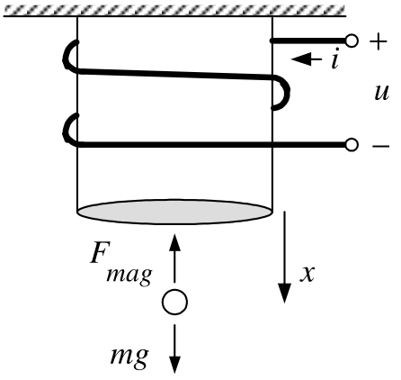
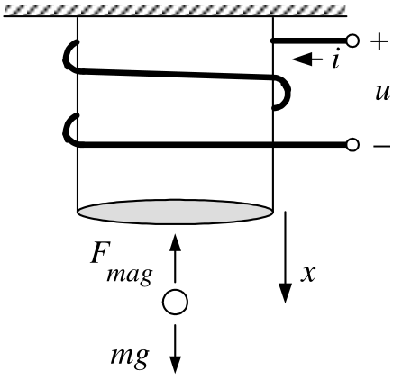
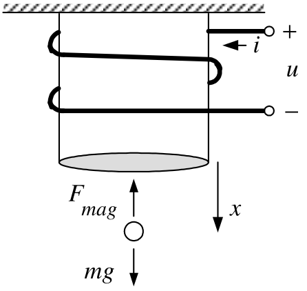
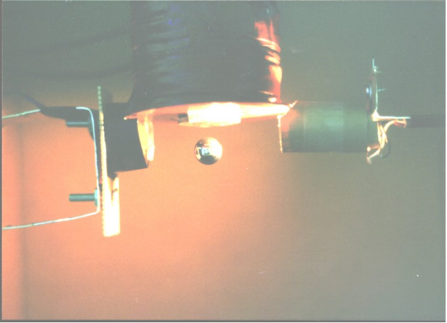
• Magnetically levitate a steel ball under an electromagnet.

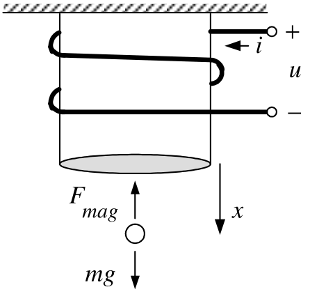
• The electromagnet consists of a wire (coil) wrapped around a core of soft iron.

• A voltage \(u\) applied to the coil produces current in the coil.

• The magnetic field of the coil’s current magnetizes the soft iron.

• The magnetized iron produces a strong magnetic field to keep a steel ball up.

• Total flux (flux linkage) in the coil windings due to the current: \(\ \lambda (x,i)\triangleq L(x)i\)

• \(L(x)=L_{0}+\dfrac{rL_{1}}{x}\) where \(x\) is the CoM of the steel ball.

  • This expression is justified later.

Mathematical Model of the Levitated Steel Ball

• Flux linkage is\(\ \lambda (x,i)\triangleq L(x)i\)  where \(L(x)=L_{0}+ \dfrac{rL_{1}}{x}.\)

• It turns out that \(L_{1}\ll L_{0}\).

• By Faraday’s law and Ohm’s law: \[u-\frac{d}{dt}\underset{\lambda }{\underbrace{\left( L(x)i\right) }}-Ri=0.\]

• Magnetic force: \[F_{mag}=-C\frac{i^{2}}{x^{2}},C\text{is a constant.}\]

Mathematical Model of the Levitated Steel Ball

DiffyQ Model: \[\begin{aligned} \frac{d}{dt}\left( L(x)i\right) +Ri &=u \\ \frac{dx}{dt} &=v \\ m\frac{dv}{dt} &=mg-C\frac{i^{2}}{x^{2}}. \end{aligned}\]

Conservation of Energy

\[\begin{aligned} \frac{d}{dt}\left( L(x)i\right) +Ri &=u \\ \frac{dx}{dt} &=v \\ m\frac{dv}{dt} &=mg-C\frac{i^{2}}{x^{2}}. \end{aligned}\]

Electrical power into the electromagnet: \[iu=i\frac{d}{dt}\left( L(x)i\right) +Ri^{2}=L(x)i\frac{di}{dt}+i^{2}\frac{ \partial L(x)}{\partial x}v+Ri^{2}.\] \(\dfrac{1}{2}L(x)i^{2}\) is the energy stored in the magnetic field of the coil & steel ball.

\(\dfrac{d}{dt}\left( \dfrac{1}{2}L(x)i^{2}\right) =L(x)i\dfrac{di}{dt}+ \dfrac{1}{2}i^{2}\dfrac{\partial L(x)}{\partial x}v.\)

Then \[\begin{aligned} iu &=\frac{d}{dt}\left( \frac{1}{2}L(x)i^{2}\right) -\frac{1}{2}i^{2}\frac{ \partial L(x)}{\partial x}v+i^{2}\frac{\partial L(x)}{\partial x}v+Ri^{2} \\ &=\frac{d}{dt}\left( \frac{1}{2}L(x)i^{2}\right) +Ri^{2}+\frac{1}{2}i^{2} \frac{\partial L(x)}{\partial x}v. \end{aligned}\]

Conservation of Energy

The electrical-power balance is \[iu=\frac{d}{dt}\left(\frac{1}{2}L(x)i^{2}\right) +Ri^{2}+\frac{1}{2}i^{2}\frac{\partial L(x)}{\partial x}v.\]

The supplied power \(iu\) goes into:

1. changing the magnetic-field energy \(\dfrac{1}{2}L(x)i^{2}\),
2. dissipation as heat \(Ri^{2}\), and
3. mechanical power \(\dfrac{1}{2}i^{2}\dfrac{\partial L(x)}{\partial x}v\).

By conservation of energy, the third term is the mechanical power supplied to the steel ball.

Using the mechanical equation gives \[\begin{aligned} m\frac{dv}{dt}&=mg-C\frac{i^{2}}{x^{2}},\\ mv\frac{dv}{dt}-mgv&=-C\frac{i^{2}}{x^{2}}v,\\ \frac{d}{dt}\left(\frac{1}{2}mv^{2}-mgx\right) &=-C\frac{i^{2}}{x^{2}}v. \end{aligned}\]

Conservation of Energy

\(V(x)=-mgx\) is the ball’s potential energy.

The rate of change of its total energy is \[\frac{d}{dt}\left(\frac{1}{2}mv^{2}+V(x)\right) =\frac{d}{dt}\left(\frac{1}{2}mv^{2}-mgx\right) =-C\frac{i^{2}}{x^{2}}v.\]

By conservation of energy, this equals the electrical power \(\dfrac{1}{2}i^{2}\dfrac{\partial L(x)}{\partial x}v\): \[\begin{aligned} \frac{1}{2}i^{2}\frac{\partial L(x)}{\partial x}v &=-C\frac{i^{2}}{x^{2}}v,\\ \frac{1}{2}i^{2}\frac{\partial}{\partial x} \left(L_{0}+\frac{rL_{1}}{x}\right)v &=-C\frac{i^{2}}{x^{2}}v,\\ -\frac{1}{2}i^{2}\frac{rL_{1}}{x^{2}}v &=-C\frac{i^{2}}{x^{2}}v,\\ C &=rL_{1}/2. \end{aligned}\]

Nonlinear Statespace Model

• Flux linkage is\(\ \lambda (x,i)\triangleq L(x)i\)  where \(L(x)=L_{0}+ \dfrac{rL_{1}}{x},\dfrac{\partial L(x)}{\partial x}=-\dfrac{rL_{1}}{x^{2}}.\)

• Magnetic Force:  \(F_{mag}=-C\dfrac{i^{2}}{x^{2}}.\)

• Conservation of Energy:  \(C=\dfrac{rL_{1}}{2}.\)

The model is now \[\begin{aligned} \frac{d\left( L(x)i\right) }{dt}+Ri=L(x)\frac{di}{dt}+i\frac{\partial L(x)}{ \partial x}v+Ri &=u \\ \frac{dx}{dt} &=v \\ m\frac{dv}{dt} &=mg-\frac{rL_{1}}{2}\frac{i^{2}}{x^{2}}. \end{aligned}\] Rearrange: \[\begin{aligned} \frac{di}{dt} &=-i\frac{1}{L(x)}\left( -\frac{rL_{1}}{x^{2}}\right) v-\frac{ R}{L(x)}i+\frac{1}{L(x)}u \\ \frac{dx}{dt} &=v \\ \frac{dv}{dt} &=g-\frac{rL_{1}}{2m}\frac{i^{2}}{x^{2}} \end{aligned}\]

Nonlinear Statespace Model

\[\begin{aligned} \frac{di}{dt} &=-i\frac{1}{L(x)}\left( -\frac{rL_{1}}{x^{2}}\right) v-\frac{ R}{L(x)}i+\frac{1}{L(x)}u \\ \frac{dx}{dt} &=v \\ \frac{dv}{dt} &=g-\frac{rL_{1}}{2m}\frac{i^{2}}{x^{2}} \end{aligned}\] The state variables are \(i,x,v\) and the state is \[\left[ \begin{array}{c} i \\ x \\ v \end{array} \right] .\] Recall \(L_{1}\ll L_{0}\) and \(x\geq r\), so \(L(x)=L_{0}+\dfrac{rL_{1}}{x}\leq L_{0}+L_{1}\approx L_{0}.\)

Replace \(L(x)\) with \(L_{0}\): \[\begin{aligned} \frac{di}{dt} &=\frac{rL_{1}}{L_{0}}\frac{i}{x^{2}}v-\frac{R}{L_{0}}i+\frac{ 1}{L_{0}}u \\ \frac{dx}{dt} &=v \\ \frac{dv}{dt} &=g-\frac{rL_{1}}{2m}\frac{i^{2}}{x^{2}}. \end{aligned}\]

Current Command Statespace Model

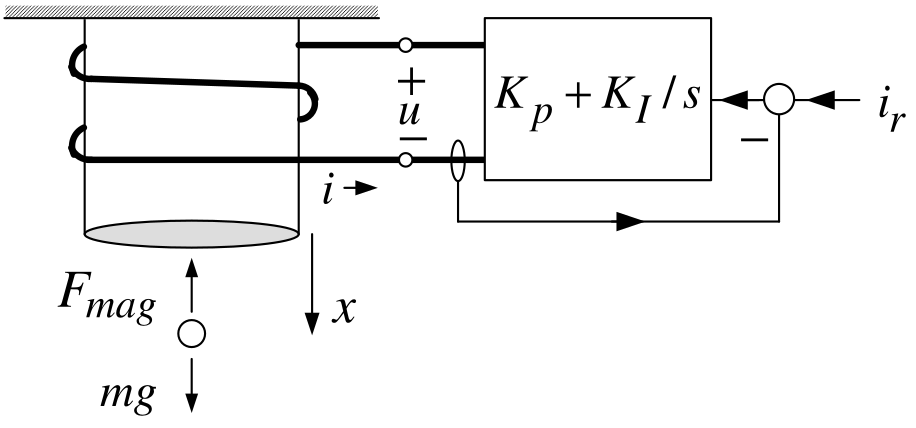
• We send a current command \(i_{r}\) to the amplifier.

• With high-gains \(K_{P},K_{I}\) the amplifier quickly forces \(i(t)\rightarrow i_{r}(t).\)

• So we can consider the current \(i(t)\) as the input. \[\begin{aligned} \frac{dx}{dt} &=v \\ \frac{dv}{dt} &=g-\frac{rL_{1}}{2m}\frac{i^{2}}{x^{2}}. \end{aligned}\]

• This is still a nonlinear statespace model.

Linearization about an Equilibrium Point

\[\begin{aligned} \frac{dx}{dt} &=v \\ \frac{dv}{dt} &=g-\frac{rL_{1}}{2m}\frac{i^{2}}{x^{2}}. \end{aligned}\]

• Let \(x=x_{eq},v=v_{eq}=0\) be the desired equilibrium point. \[\begin{aligned} \frac{dx_{eq}}{dt} &=v_{eq} \\ \frac{dv_{eq}}{dt} &=g-\frac{rL_{1}}{2m}\frac{i_{eq}^{2}}{x_{eq}^{2}}. \end{aligned}\]

• The \(1^{st}\) eqn holds because \(x_{eq}\) is a constant and \(v_{eq}=0\).

• The 2\(^{nd}\) eqn requires \(g=\dfrac{rL_{1}}{2m}\dfrac{i_{eq}^{2}}{ x_{eq}^{2}}\) or \[i_{eq}=x_{eq}\sqrt{\dfrac{2mg}{rL_{1}}}.\]

Linearization about an Equilibrium Point

\[\begin{aligned} \frac{dx}{dt}&=v,\\ \frac{dv}{dt}&=f(x,i) =g-\frac{rL_{1}}{2m}\frac{i^{2}}{x^{2}}. \end{aligned}\]

Let \[\Delta x\triangleq x-x_{eq},\qquad \Delta i\triangleq i-i_{eq}.\]

Dropping higher-order terms, the Taylor expansion becomes \[\begin{aligned} f(x,i) &\approx f(x_{eq},i_{eq}) +\left.\frac{\partial f}{\partial x}\right|_{eq}\Delta x +\left.\frac{\partial f}{\partial i}\right|_{eq}\Delta i\\ &=0 +\frac{rL_{1}}{m}\frac{i_{eq}^{2}}{x_{eq}^{3}}\Delta x -\frac{rL_{1}}{m}\frac{i_{eq}}{x_{eq}^{2}}\Delta i\\ &=\frac{2g}{x_{eq}}\Delta x -\frac{2g}{i_{eq}}\Delta i. \end{aligned}\]

Here \[\frac{rL_{1}}{m}\frac{i_{eq}^{2}}{x_{eq}^{3}} =\frac{2g}{x_{eq}}, \qquad \frac{rL_{1}}{m}\frac{i_{eq}}{x_{eq}^{2}} =\frac{2g}{i_{eq}}.\]

Linear Statespace Model

\[\begin{aligned} \dfrac{dx}{dt} &=v \\ \dfrac{dv}{dt} &=\frac{2g}{x_{eq}}(x-x_{eq})-\frac{2g}{i_{eq}}(i-i_{eq}). \end{aligned}\] \(\dfrac{dv_{eq}}{dt}=0,\dfrac{dx_{eq}}{dt}=0\Longrightarrow\) \[\begin{aligned} \frac{d}{dt}(x-x_{eq}) &=v-v_{eq} \\ \frac{d}{dt}(v-v_{eq}) &=\frac{2g}{x_{eq}}(x-x_{eq})-\frac{2g}{i_{eq}} (i-i_{eq}). \end{aligned}\]

Set \(\Delta x\triangleq x-x_{eq},\Delta v\triangleq v-v_{eq},\Delta i\triangleq i-i_{eq}\): \[\begin{aligned} \frac{d}{dt}\Delta x &=\Delta v \\ \frac{d}{dt}\Delta v &=\frac{2g}{x_{eq}}\Delta x-\frac{2g}{i_{eq}}\Delta i \end{aligned}\] or \[\frac{d}{dt}\left[ \begin{array}{c} \Delta x \\ \Delta v \end{array} \right] =\underset{A}{\underbrace{\left[ \begin{array}{cc} 0 & 1 \\ \dfrac{2g}{x_{eq}} & 0 \end{array} \right] }}\left[ \begin{array}{c} \Delta x \\ \Delta v \end{array} \right] +\underset{b}{\underbrace{\left[ \begin{array}{c} 0 \\ -\dfrac{2g}{i_{eq}} \end{array} \right] }}\Delta i.\]

Linear Statespace Model

\[\frac{d}{dt}\left[ \begin{array}{c} \Delta x \\ \Delta v \end{array} \right] =\underset{A}{\underbrace{\left[ \begin{array}{cc} 0 & 1 \\ \dfrac{2g}{x_{eq}} & 0 \end{array} \right] }}\left[ \begin{array}{c} \Delta x \\ \Delta v \end{array} \right] +\underset{b}{\underbrace{\left[ \begin{array}{c} 0 \\ -\dfrac{2g}{i_{eq}} \end{array} \right] }}\Delta i.\] More compactly:

\[\frac{d}{dt}\left[ \begin{array}{c} \Delta x \\ \Delta v \end{array} \right] =A\left[ \begin{array}{c} \Delta x \\ \Delta v \end{array} \right] +b\Delta i\]

• This is a linear statespace model.

• \(\Delta x=x-x_{eq}\) and \(\Delta v=v-v_{eq}\) are the state variables.

• \(\Delta i=i-i_{eq}\) is the input.

Transfer Function Model

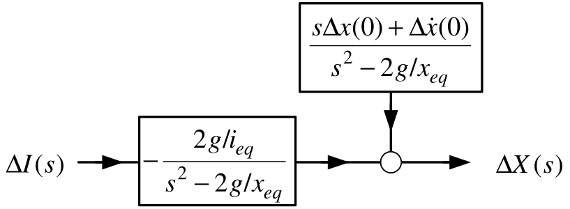
\[\begin{aligned} \frac{d}{dt}\left[ \begin{array}{c} \Delta x \\ \Delta v \end{array} \right] &=\underset{A}{\underbrace{\left[ \begin{array}{cc} 0 & 1 \\ \dfrac{2g}{x_{eq}} & 0 \end{array} \right] }}\left[ \begin{array}{c} \Delta x \\ \Delta v \end{array} \right] +\underset{b}{\underbrace{\left[ \begin{array}{c} 0 \\ -\dfrac{2g}{i_{eq}} \end{array} \right] }}\Delta i \\ \Longrightarrow \frac{d\Delta v}{dt} &=\frac{d^{2}}{dt^{2}}\Delta x=\frac{2g }{x_{eq}}\Delta x-\frac{2g}{i_{eq}}\Delta i. \end{aligned}\] Laplace transform: \[s^{2}\Delta X(s)-s\Delta x(0)-\Delta \dot{x}(0)=\frac{2g}{x_{eq}}\Delta X(s)- \frac{2g}{i_{eq}}\Delta I(s)\] or \[\Delta X(s)=\underset{\text{transfer function}}{\underbrace{-\frac{\dfrac{2g }{i_{eq}}}{s^{2}-\dfrac{2g}{x_{eq}}}}}\Delta I(s)+\frac{s\Delta x(0)+\Delta \dot{x}(0)}{s^{2}-\dfrac{2g}{x_{eq}}}.\]

• Note the similarity to the transfer function of the inverted pendulum!

• The TF has poles at \(\pm \sqrt{\dfrac{2g}{x_{eq}}}\) and is therefore unstable.

Block Diagram of the Transfer Function Model

\[\Delta X(s)=\underset{\text{transfer function}}{\underbrace{-\frac{2g/i_{eq} }{s^{2}-2g/x_{eq}}}}\Delta I(s)+\frac{s\Delta x(0)+\Delta \dot{x}(0)}{ s^{2}-2g/x_{eq}}.\]

Cart on a Track System

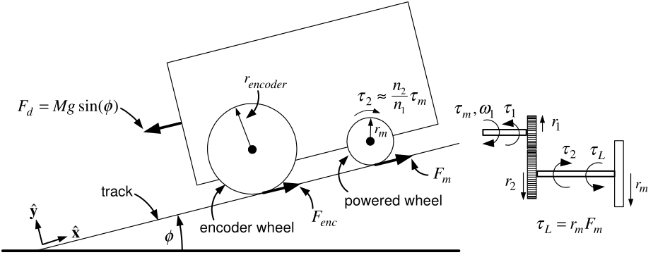
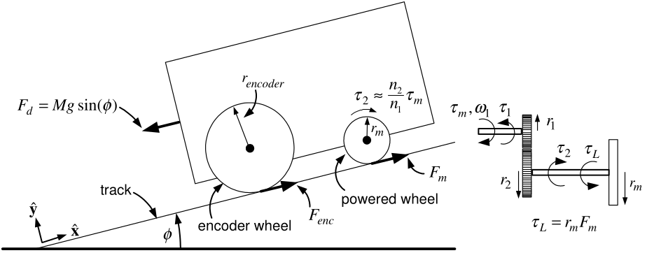
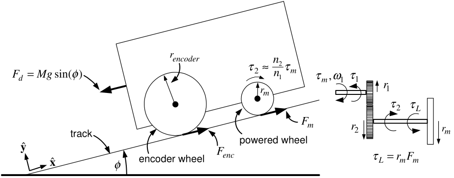
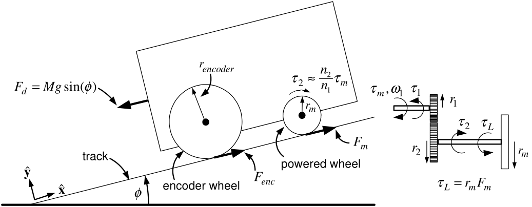
Motor shaft with gear 1 has moment of inertia \(J_{1}.\)

Wheel shaft with gear 2 has moment of inertia \(J_{2}\).

\(\quad F_{m}\mathbf{\hat{x}}\) is the force exerted on the powered wheels by the track.

\(-F_{m}\mathbf{\hat{x}}\) is the force exerted on the track by the powered wheels.

\(\quad\)Set \(F_{enc}=0\) as it is neglible.

\(\quad \tau _{1}\) is the torque exerted on gear 1 by gear 2

\(\quad \tau _{2}\) is the (reaction) torque exerted on gear 2 by gear 1.

Cart on a Track System

Mechanical Equations

\[\begin{aligned} J_{1}\frac{d\omega _{1}}{dt} &=\tau _{m}-\tau _{1} \\ J_{2}\frac{d\omega _{2}}{dt} &=\tau _{2}-r_{m}F_{m} \end{aligned}\]

Use \(\omega _{1}=\dfrac{n_{2}}{n_{1}}\omega _{2}\) and \(\tau _{2}=\dfrac{ n_{2}}{n_{1}}\tau _{1}\) to obtain \[\underset{J}{\underbrace{\left( J_{1}\left( \frac{n_{2}}{n_{1}}\right) ^{2}+J_{2}\right) }}\frac{d\omega _{2}}{dt}=\frac{n_{2}}{n_{1}}\tau _{m}-F_{m}r_{m}\]

Cart on a Track System

Mechanical Equations

\[\begin{aligned} J\frac{d\omega _{2}}{dt} &=\frac{n_{2}}{n_{1}}\tau _{m}-F_{m}r_{m} \\ M\frac{dv}{dt} &=F_{m}-F_{d}. \end{aligned}\] No slip condition \(\ r_{enc}\omega _{enc}=r_{m}\omega _{2}=v.\)

With \(\omega _{2}=v/r_{m}\) and eliminating \(F_{m}\) we have \[\left( \frac{J}{r_{m}^{2}}+M\right) \frac{dv}{dt}=\frac{1}{r_{m}}\frac{n_{2} }{n_{1}}\tau _{m}-F_{d}.\]

Cart on a Track System

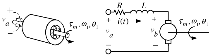
Electrical Equations

 

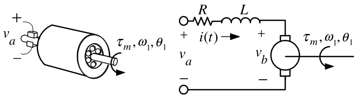
\[\begin{aligned} L\frac{di}{dt} &=-Ri(t)-K_{b}\omega _{1}(t)+v_{a}(t) \\ \tau _{m} &=K_{T}i(t). \end{aligned}\]

Cart on a Track System

Electrical Equations

\[\begin{aligned} L\frac{di}{dt} &=-Ri(t)-K_{b}\omega _{1}(t)+v_{a}(t) \\ \tau _{m} &=K_{T}i(t). \end{aligned}\] With \(\omega _{1}=\dfrac{n_{2}}{n_{1}}\omega _{2}=\dfrac{n_{2}}{n_{1}}\dfrac{ v}{r_{m}}\) we have \[\begin{aligned} L\frac{di}{dt} &=-Ri(t)-\underset{v_{b}(t)}{\underbrace{\frac{K_{b}}{r_{m}} \frac{n_{2}}{n_{1}}v(t)}}+v_{a}(t) \\ \tau _{m} &=K_{T}i(t). \end{aligned}\]

Cart on a Track System

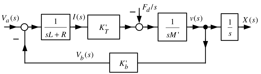
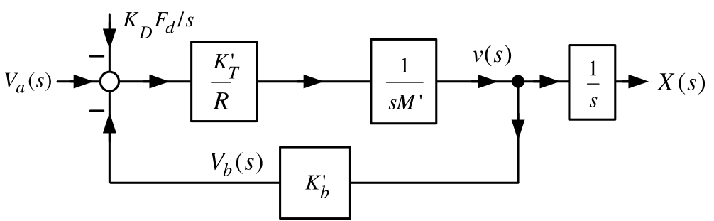
Equations of Motion \[\begin{aligned} L\frac{di}{dt} &=-Ri(t)-\frac{K_{b}}{r_{m}}\frac{n_{2}}{n_{1}}v(t)+v_{a}(t) \left( \frac{J}{r_{m}^{2}}+M\right) \frac{dv}{dt} &=\left( \frac{n_{2}}{ n_{1}}\frac{1}{r_{m}}\right) K_{T}i(t)-F_{d} \\ \frac{dx}{dt} &=v. \end{aligned}\] Laplace Transform \[\begin{aligned} I(s) &=\frac{V_{a}(s)-V_{b}(s)}{sL+R} \\ V_{b}(s) &=\underset{K_{b}^{\prime }}{\underbrace{K_{b}\frac{n_{2}}{n_{1}} \frac{1}{r_{m}}}}v(s) \\ s\underset{M^{\prime }}{\underbrace{\left( \frac{J}{r_{m}^{2}}+M\right) }} v(s) &=\underset{K_{T}^{\prime }}{\underbrace{\frac{n_{2}}{n_{1}}\frac{1}{ r_{m}}K_{T}}}I(s)-\frac{F_{d}}{s}. \end{aligned}\]

Cart on a Track System

• \(K_{T}^{\prime }\triangleq K_{T}\dfrac{n_{2}}{n_{1}}\dfrac{1}{r_{m}},\)  \(K_{b}^{\prime }\triangleq K_{b}\dfrac{n_{2}}{n_{1}}\dfrac{1}{r_{m}},\)  \(M^{\prime }\triangleq \dfrac{J}{r_{m}^{2}}+M\)

  

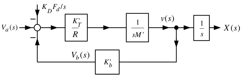
• Set \(L=0\)  and \(K_{D}\triangleq \dfrac{R}{K_{T}^{\prime }}=\dfrac{R}{ K_{T}\dfrac{n_{2}}{n_{1}}\dfrac{1}{r_{m}}}\)

  

Cart on a Track System

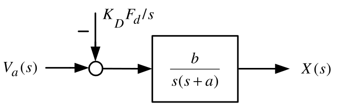
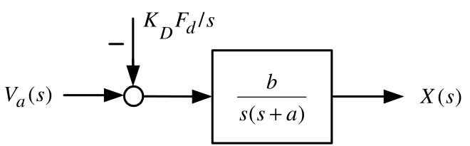
Define \[G(s)\triangleq \frac{\dfrac{K_{T}^{\prime }}{R}\dfrac{1}{sM^{\prime }}}{ 1+K_{b}^{\prime }\dfrac{K_{T}^{\prime }}{R}\dfrac{1}{sM^{\prime }}}\frac{1}{s }=\frac{K_{T}^{\prime }}{sRM^{\prime }+K_{b}^{\prime }K_{T}^{\prime }}\frac{1 }{s}=\frac{\dfrac{K_{T}^{\prime }}{RM^{\prime }}}{s+\dfrac{K_{b}^{\prime }K_{T}^{\prime }}{RM^{\prime }}}\frac{1}{s}=\frac{b}{s\left( s+a\right) }\]

Simplified block diagram

Cart on a Track System

\[X(s)=\frac{b}{s\left( s+a\right) }V_{a}(s)-\frac{b}{s\left( s+a\right) }K_{D} \frac{F_{d}}{s}.\]

• \(K_{D}F_{d}\) is an input voltage disturbance.

• Equivalent to the actual disturbance \(F_{d}\).

• \(K_{D}F_{d}=\dfrac{R}{K_{T}\dfrac{n_{2}}{n_{1}}\dfrac{1}{r_{m}}}F_{d}= \dfrac{n_{2}}{n_{1}}\dfrac{r_{m}F_{D}}{K_{T}}R\) has units of Volts.

• \(bK_{D}F_{d}=\dfrac{K_{T}^{\prime }}{RM^{\prime }}\dfrac{R}{ K_{T}^{\prime }}Mg\sin (\phi )=\dfrac{Mg\sin (\phi )}{M^{\prime }}=\dfrac{ Mg\sin (\phi )}{J/r_{m}^{2}+M}\). \[\frac{d^{2}x(t)}{dt^{2}}=-ax(t)+bv_{a}(t)-\dfrac{Mg\sin (\phi )}{ J/r_{m}^{2}+M}u_{s}(t).\]