Root Locus
System Modeling and Control · Chapter 12
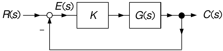
Let \(G(s)\) be given by \[G(s)=\frac{b(s)}{a(s)}=\frac{b_{m}s^{m}+b_{m-1}s^{m-1}+\cdots+b_{1}s+b_{0}}{s^{n}+a_{n-1}s^{n-1}+\cdots+a_{1}s+a_{0}},\text{ }m<n\] The closed-loop transfer function is \[\frac{C(s)}{R(s)}=\frac{KG(s)}{1+KG(s)}=\frac{Kb(s)\!/\!a(s)}{1+Kb(s)\!/\!a(s)}=\frac{Kb(s)}{a(s)+Kb(s)}.\]
As \(K\) is varied from \(0\) to \(\infty\) we want to know the location of the roots of \[a(s)+Kb(s)=0.\]
\(a(s)+Kb(s)\) is the closed-loop characteristic polynomial.
The roots of \(a(s)+Kb(s)=0\) are the closed-loop poles.
The root locus is a plot of the roots of \(a(s)+Kb(s)=0\) as \(K\) goes from \(0\) to \(\infty.\)
From previous slide: \[p_{1},p_{2}=\left\{ \begin{array}{ll} -2+\sqrt{4-K},\text{ }-2-\sqrt{4-K}, & 0\leq K\leq4 \\ & \\ -2\pm j\sqrt{K-4}, & 4\leq K.\end{array} \right.\]
For \(K=0,2,4,8\) we have\[\begin{array}{|c|c|} \hline K & p_{1},p_{2} \\ \hline 0 & 0,-4 \\ \hline 2 & -2+\sqrt{2},-2-\sqrt{2} \\ \hline 4 & -2,-2 \\ \hline 8 & -2\pm j2 \\ \hline \end{array}\]
Sketch the root locus.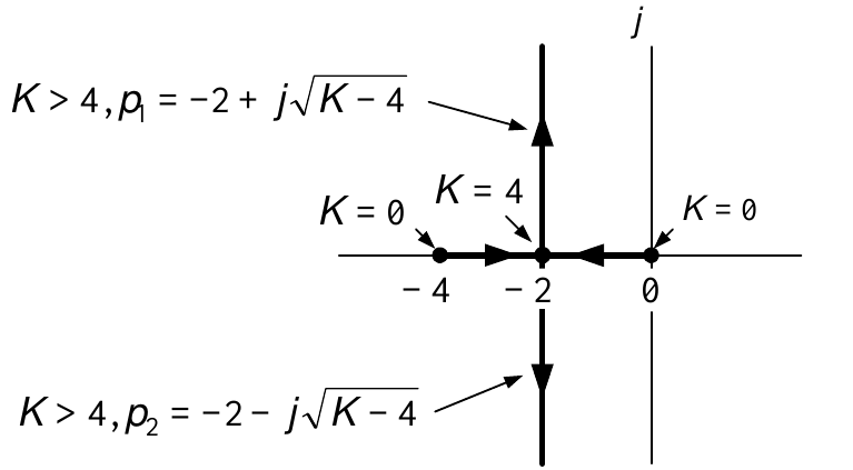
\[\begin{aligned} G(s) & =\dfrac{1}{s(s+4)}=\dfrac{1}{\underset{s}{\underbrace{|s|e^{j\angle s}}}\text{ }\underset{s+4}{\underbrace{|s+4|e^{j\angle(s+4)}}}}=\dfrac {1}{|s||s+4|}e^{-j\angle s}e^{-j\angle(s+4)} \\ & \\ \Longrightarrow\text{ }\angle G(s) & =-\angle s-\angle(s+4). \end{aligned}\]
Let the point “\(s\)” be on the root locus.
\(s+4=s-(-4)\) is a vector from \(-4\) to \(s.\)
\(s\) is a vector from \(0\) to \(s.\)
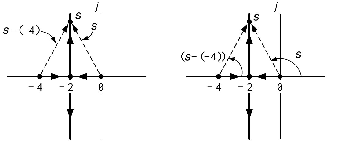
The figure shows \(\angle s+\angle(s+4)=\pi,\) i.e., \[\angle G(s)=-\angle s-\angle(s+4)=-\pi.\]
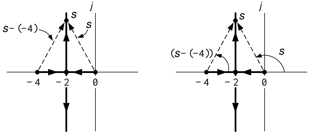
For example, \(s=-2+2j\) is on the root locus and \[\begin{aligned} G(-2+2j) & =\dfrac{1}{(-2+j2)(-2+2j+4)}=\frac{1}{(-2+2j)(2+2j)}=-\frac{1}{8} \\ & \\ \Longrightarrow\angle G(-2+2j) & =\angle(-1/8)=\pi. \end{aligned}\]
On the other hand \(s=-4+2j\) is not on the root locus and \[\begin{aligned} G(-4+2j) & =\dfrac{1}{(-4+j2)(-4+2j+4)}=\frac{1}{(-4+2j)(2j)}=-\frac {1}{4+8j} \\ & \\ \Longrightarrow\angle G(-4+2j) & \neq\pi(2\ell+1),\text{ }\ell=0,\pm 1,\pm2,..... \end{aligned}\]
(5) A breakaway point occurs at \(s=-2\) for \(K=4.\)
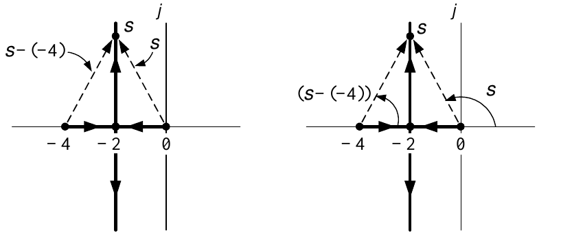
This is where \(a(s)+Kb(s)=s^{2}+4s+K=0\) has a double root, that is, \[\left. 1+K\frac{1}{s(s+4)}\right\vert _{K=4}=\left. \dfrac{s^{2}+4s+K}{s(s+4)}\right\vert _{K=4}=\dfrac{(s+2)^{2}}{s(s+4)}\]
\[\begin{aligned} \!\!\!\!\!\!\!\left. \frac{d}{ds}\left( 1+4\frac{1}{s(s+4)}\right) \right\vert _{s=-2}\!\!\!\!\!\!\! & =\!\!\!\!\left. \frac{d}{ds}\left( \dfrac{(s+2)^{2}}{s(s+4)}\right) \right\vert _{s=-2} \\ \!\!\!\!\!\!\! & =\!\!\!\!\left. -\dfrac{1}{s(s+4)}\left( \dfrac{d}{ds}(s^{2}+4s)\right) (s+2)^{2}\right\vert _{s=-2}\!\!\!\!+\left. \left( \dfrac{1}{s(s+4)}\dfrac{d}{ds}(s+2)^{2}\right) \right\vert _{s=-2} \\ \!\!\!\!\!\!\! & =\!\!\!\!0. \end{aligned}\]
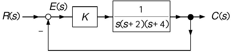
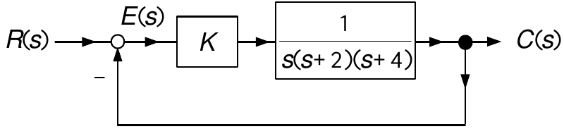
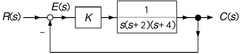
\(G(s)=\dfrac{1}{s(s+2)(s+4)}=\dfrac{1}{|s||s+2||s+4|}e^{-j\left( \angle s+\angle(s+2)+\angle(s+4)\right) }.\)
\(1+KG(s)=1+K\dfrac{1}{s(s+2)(s+4)}=\dfrac{s(s+2)(s+4)+K}{s(s+2)(s+4)}=0.\)
\(G(s)=-\dfrac{1}{K}\Longrightarrow\angle G(s)=\pi(2\ell+1),\ell =0,\pm1,\pm2,....\)
Sketch the root locus.
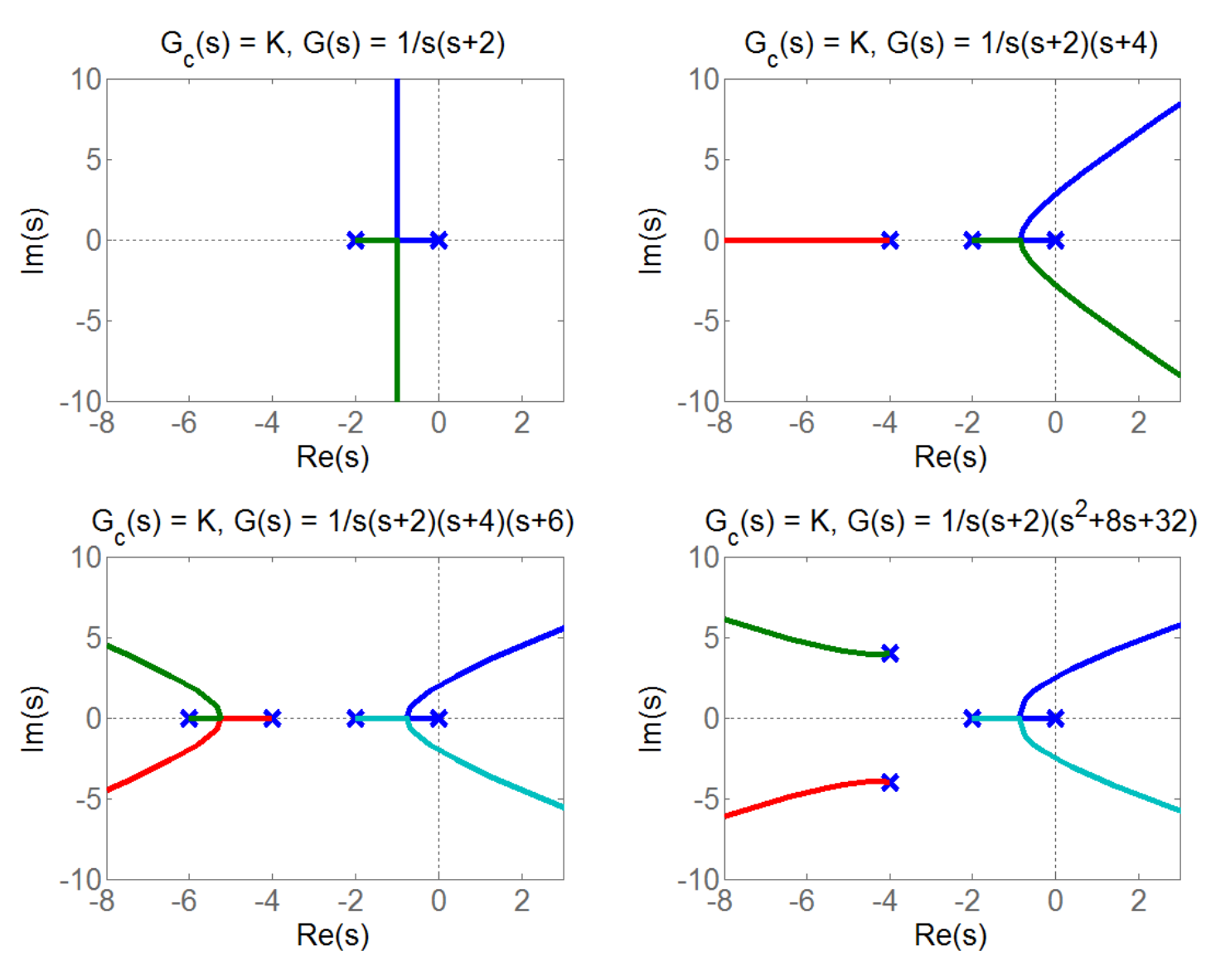
(1) With \(K=0\) we have \(s(s+2)(s+4)+K=s(s+2)(s+4)=0\) or \(s=0,-2,-4.\)
- The root locus starts on the open-loop poles.
(2) \(1+KG(s)=0\) or \(G(s)=\dfrac{1}{s(s+2)(s+4)}=-\dfrac{1}{K}.\)
- As \(K\rightarrow\infty,\) the 3 roots go to infinity, i.e., \(|s|\rightarrow\infty.\)
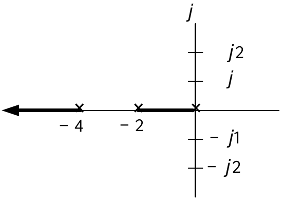
(i) Consider \(s\) real with \(-2<s<0\) so \(\angle s=\pi,\angle (s+2)=0,\angle(s+4)=0.\)
Then \[\angle G(s)=-\angle s-\angle(s+2)-\angle(s+4)=-\pi.\]
These values of \(s\) are on the root locus.
(ii) Consider \(s\) real with \(-4<s<-2\) so \(\angle s=\pi,\angle (s+2)=\pi,\angle(s+4)=0.\)
Then \[\angle G(s)=-\angle s-\angle(s+2)-\angle(s+4)=-2\pi.\]
These values of \(s\) are not on the root locus.
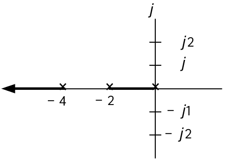
(iii) Consider \(s\) real with \(s<-4\) so \(\angle s=\pi,\angle (s+2)=\pi,\angle(s+4)=\pi.\)
Then \[\angle G(s)=-\angle s-\angle(s+2)-\angle(s+4)=-3\pi.\]
These values of \(s\) are on the root locus.
(iv) Finally, consider \(s\) real with \(s>0\) so \(\angle s=0,\angle (s+2)=0,\angle(s+4)=0.\)
Then \[\angle G(s)=-\angle s-\angle(s+2)-\angle(s+4)=0.\]
These values of \(s\) are not on the root locus.
(4) Breakaway Point (continued) \[\begin{aligned} \frac{d}{ds}G(s) & =-\left( \dfrac{1}{s(s+2)(s+4)}\right) ^{2}\frac{d}{ds}\left( s(s+2)(s+4)\right) \\ & =-\left( \dfrac{1}{s(s+2)(s+4)}\right) ^{2}\frac{d}{ds}\left( s^{3}+6s^{2}+8s\right) . \end{aligned}\]
\(\dfrac{d}{ds}G(s)=0\) requires solving \(3s^{2}+12s+8=0\) \(\Longrightarrow\) \[s=\frac{-12\pm\sqrt{(12)^{2}-4(3)(8)}}{6}=-2\pm\frac{2}{\sqrt{3}}=-0.845,-3.146\]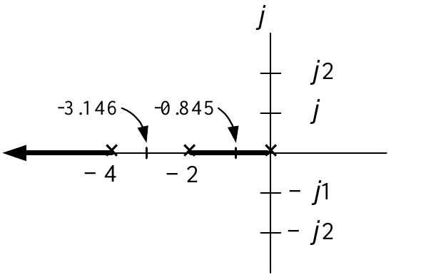
Only \(s=-0.845\) is on the real axis root locus and is therefore the only breakaway point.
(5) \(j\omega\) axis intercepts
Apply the Routh-Hurwitz test to \[s(s+2)(s+4)+K=s^{3}+6s^{2}+8s+K.\] The Routh table is\[\begin{array}{cccccc} s^{3} & & 1 & & 8 & \\ s^{2} & & 6 & & K & \\ s & & (48-K)/6 & & 0 & \\ 1 & & K & & & \end{array}\]
Stable for \(0<K<48.\)
Two right half-plane poles for \(K>48.\)
\(\Longrightarrow\) At \(K=48\) there are two poles on the \(j\omega\) axis.
To find these poles solve the auxiliary equation \(6s^{2}+48=0\) to obtain \(s=\pm j2\sqrt{2}=\pm j2.83.\)
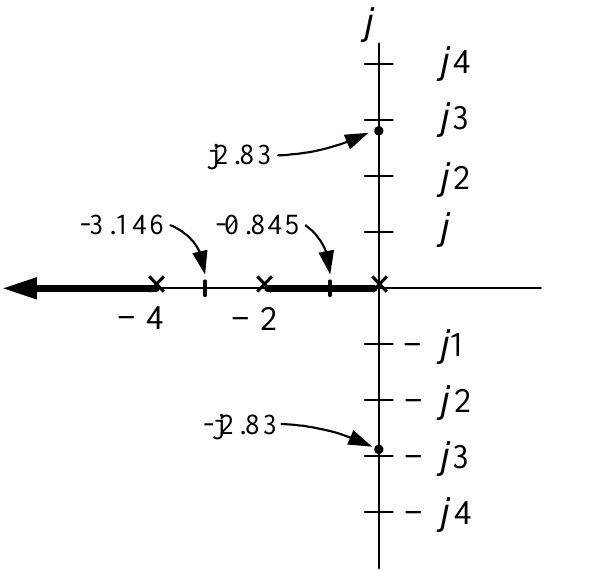
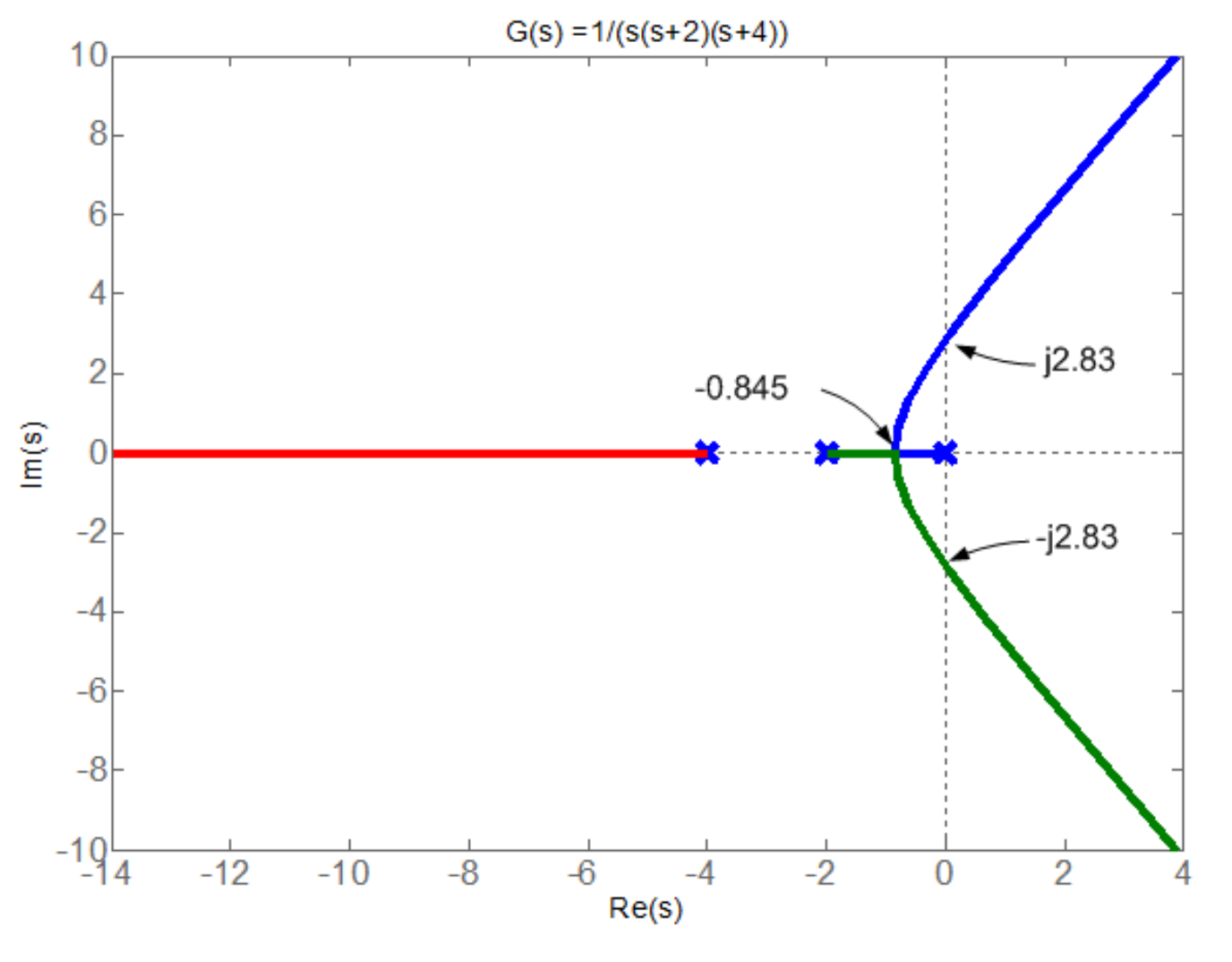
Using the above results we (Matlab!) can sketch the root locus as shown below.
Then the angles of the asymptotes with respect to the real axis are (\(n=3,m=0\)) \[\begin{aligned} \theta_{\ell} & =\frac{(2\ell+1)\pi}{3-0},\ell=0,1,2 \\ & =\frac{\pi}{3},\frac{3\pi}{3},\frac{5\pi}{3} \\ & =\frac{\pi}{3},\pi,-\frac{\pi}{3} \end{aligned}\] and these asymptotes intersect at\[\begin{aligned} \sigma_{1} & =-\frac{a_{n-1}-0}{n-m},\text{ }n=3,m=0 \\ & =-\frac{6-0}{3-0},\text{ }a_{2}=6 \\ & =-2. \end{aligned}\]
\(\theta_{\ell}=\dfrac{\pi}{3},\pi,-\dfrac{\pi}{3}\) and \(\sigma_{1}=-2.\)
The asymptotes intersect the \(j\omega\) axis at \(\pm j2\tan(\pi/3)=\pm2\sqrt {3}=\pm j3.46.\)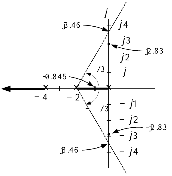
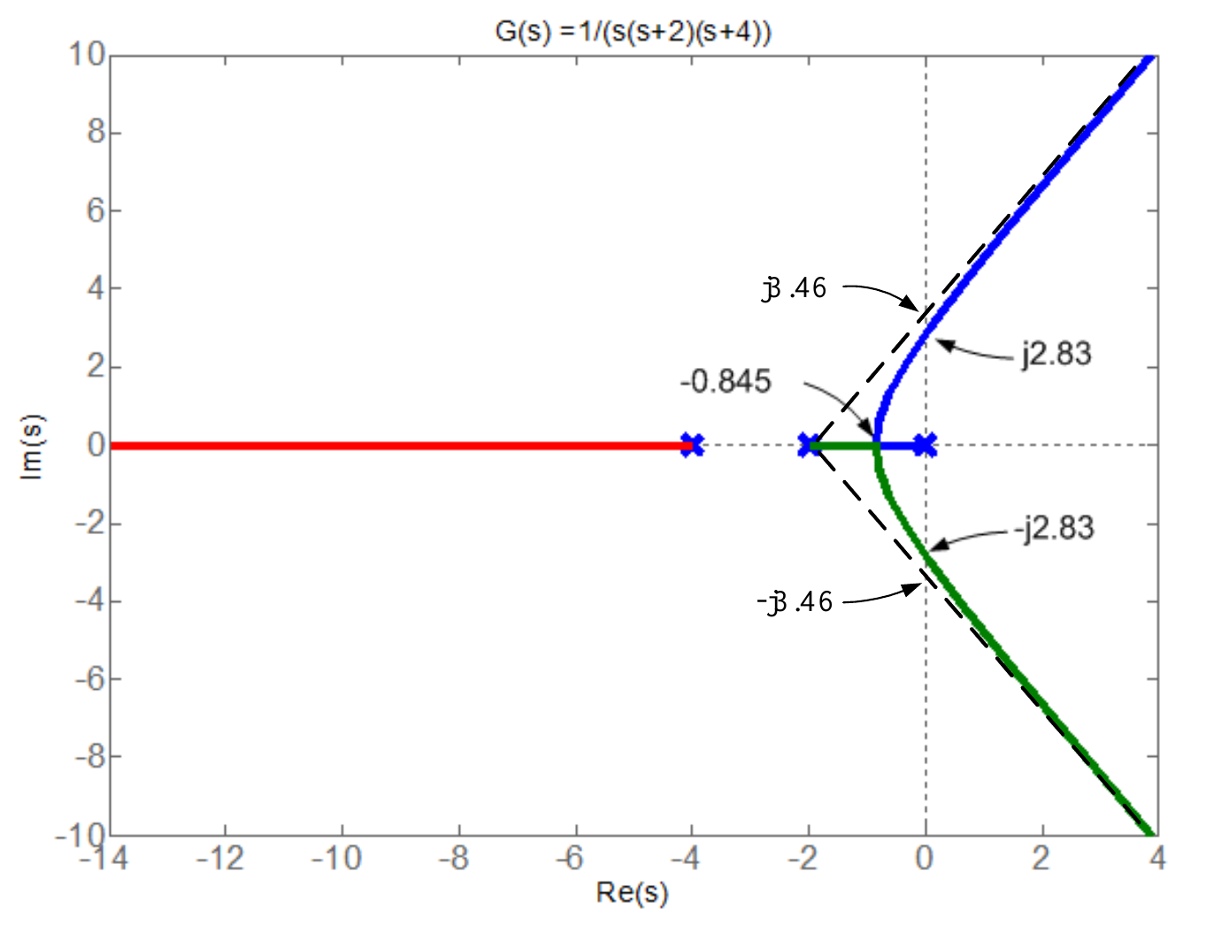
- Matlab plot of the root locus (See slide ).
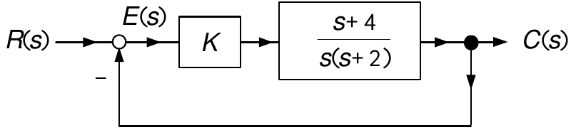
Return Difference
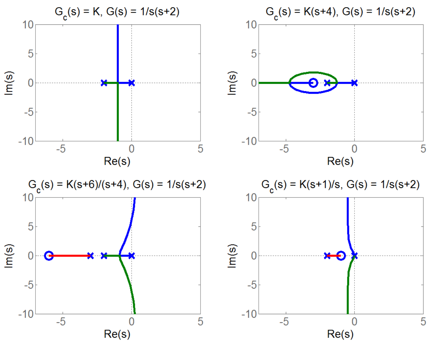
\[1+KG(s)=1+K\dfrac{s+4}{s(s+2)}=\dfrac{s(s+2)+K(s+4)}{s(s+2)}\] Angle Condition \(G(s)=-\dfrac{1}{K}\) \(\Longrightarrow\) \[\angle(s+4)-\angle s-\angle(s+2)=\pi(2\ell+1),\ell=0,\pm 1,\pm2,....\]
(1) \(K=0.\) Then \(s(s+2)+K(s+4)=s(s+2)=0\) \(\Longrightarrow\) \(\ s=0,-2.\)
(2) \(K=\infty.\) From \(G(s)=\dfrac{s+4}{s(s+2)}=-\dfrac{1}{K}\) \(\ \Longrightarrow\) \(s\rightarrow-4\) or \(|s|\rightarrow\infty\) as \(K\rightarrow\infty\).
\(G(s)\) has one zero at \(-4\) and one zero at \(|s|=\infty\).
The root locus ends on the open-loop zeros.
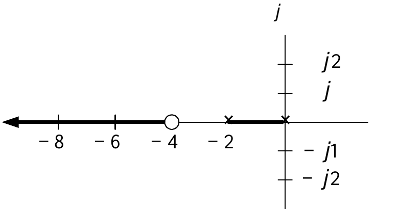
(3) Real Axis Root Locus
(i) Consider \(s\) real with \(-2<s<0\) so \(\angle s=\pi,\angle (s+2)=0,\angle(s+4)=0.\)
Then \[\angle G(s)=\angle(s+4)-\angle s-\angle(s+2)=-\pi.\]
These values of \(s\) are on the root locus.
(ii) Consider \(s\) real with \(-4<s<-2\) so \(\angle s=\pi,\angle (s+2)=\pi,\angle(s+4)=0.\)
Then \[\angle G(s)=\angle(s+4)-\angle s-\angle(s+2)=0.\]
These values of \(s\) are not on the root locus.
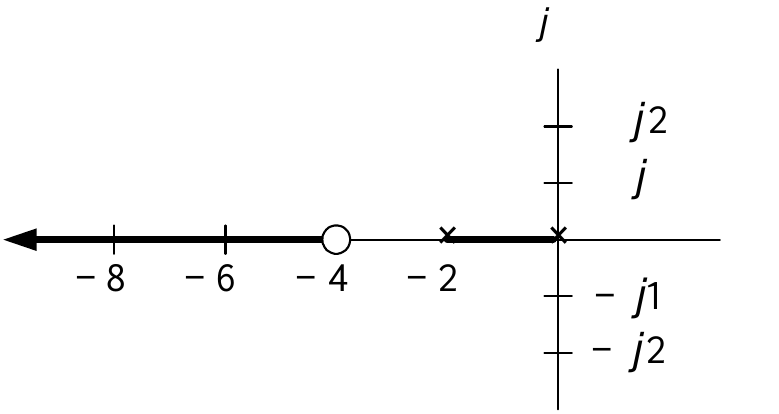
(3) Real Axis Root Locus (continued)
(iii) Consider \(s\) real with \(s<-4\) so \(\angle s=\pi,\angle (s+2)=\pi,\angle(s+4)=\pi.\)
Then \[\angle G(s)=\angle(s+4)-\angle s-\angle(s+2)=-\pi.\]
These values of \(s\) are on the root locus.
(iv) Finally, consider \(s\) real with \(s>0\) so \(\angle s=0,\angle (s+2)=0,\angle(s+4)=0.\)
Then \[\angle G(s)=-\angle s-\angle(s+2)-\angle(s+4)=0.\]
These values of \(s\) are not on the root locus.
Breakaway Point
Solve \[\frac{d}{ds}\underset{G(s)}{\underbrace{\left( \dfrac{s+4}{s(s+2)}\right) }}=0.\]
\[\frac{d}{ds}G(s)=\dfrac{1}{s(s+2)}-\dfrac{s+4}{\left[ s(s+2)\right] ^{2}}\frac{d}{ds}\left( s^{2}+2s\right) =\frac{s(s+2)-(s+4)(2s+2)}{\left[ s(s+2)\right] ^{2}}=-\frac{s^{2}+8s+8}{\left[ s(s+2)\right] ^{2}}\]
\(\dfrac{d}{ds}G(s)=0\) requires \(s^{2}+8s+8=0\), or \[s=\frac{-8\pm\sqrt{64-32}}{2}=-4\pm2\sqrt{2}=-6.828,-1.172\]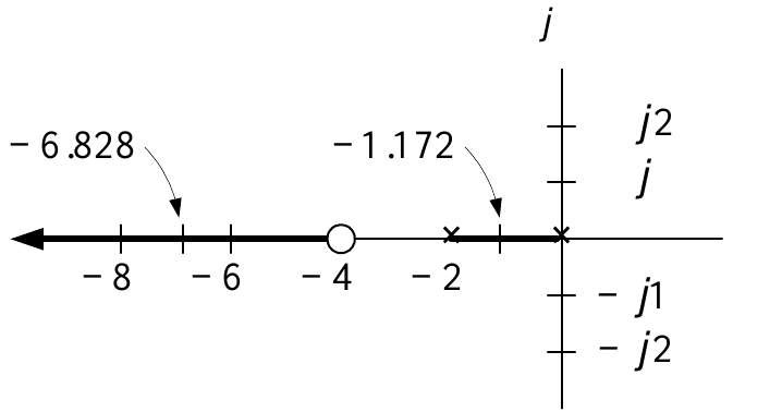
- Both roots of \(dG/ds=0\) are on the real axis root locus and so are breakaway pts.
Sketch Previously
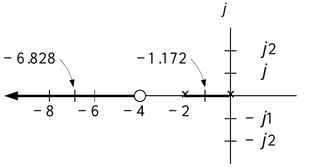
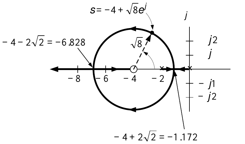
Using the angle condition we show that the root locus that is off the real axis is a circle!
\(G(s)=\dfrac{1}{s(s^{2}+2s+2)}=\dfrac{|s+4|}{|s||s-(-1+j)||s-(-1-j)|}e^{-j\left( \angle s+\angle(s-(-1+j))+\angle s-(-1-j)\right) }.\)
The denominator \(G(s)\) factors as \(s(s^{2}+2s+2)=s[s-(-1+j)][s-(-1-j)].\)
The pair of complex conjugate open-loop poles leads to the angles of departure.
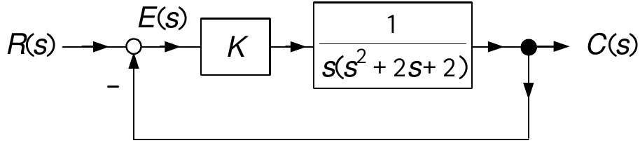
The closed-loop poles are the zeros of \[1+KG(s)=1+K\dfrac{1}{s(s^{2}+2s+2)}=\dfrac{s^{3}+2s^{2}+2s+K}{s(s^{2}+2s+2)}.\] By the angle condition CL poles satisfy \[G(s)=-\frac{1}{K}\text{ }\Longrightarrow\angle G(s)=\pi(2\ell+1),\ell =0,\pm1,\pm2,....\] or \[-\angle s-\angle\lbrack(s-(-1+j)]-\angle\lbrack s-(-1-j)]=\pi (2\ell+1),\ell=0,\pm1,\pm2,....\]
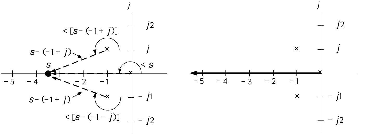
(i) \(s\) real with \(-\infty<s<0\) so \(\angle s=\pi,\angle \lbrack(s-(-1+j)]=-\angle\lbrack(s-(-1-j)]\). \[\angle G(s)=-\angle s\underset{0}{\underbrace{-\angle \lbrack(s-(-1+j)]-\angle\lbrack s-(-1-j)]}}\text{ }=-\angle s=-\pi\]
These values of \(s\) are on the root locus.
(ii) \(s\) real with \(s>0\) so \(\angle s=0,\angle\lbrack (s-(-1+j)]=-\angle\lbrack(s-(-1-j)].\) \[\angle G(s)=-\angle s\underset{0}{\underbrace{-\angle \lbrack(s-(-1+j)]-\angle\lbrack s-(-1-j)]}}\text{ }=-\angle s=0\]
These values of \(s\) are not on the root locus.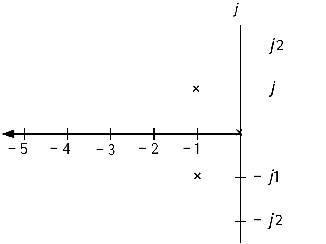
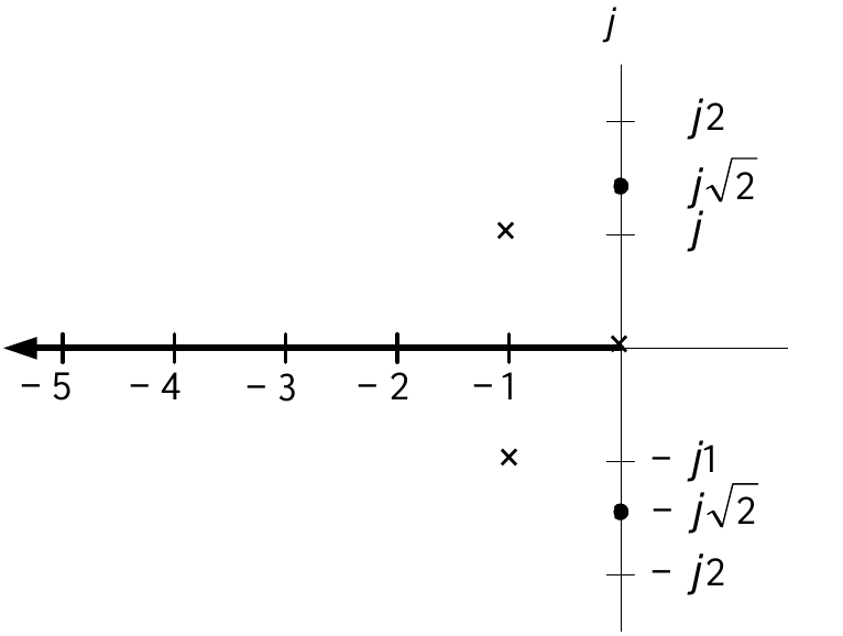
(5) \(j\omega\) axis intercepts The Routh table for \(s^{3}+2s^{2}+2s+K=0\) is \[\begin{array}{cccccc} s^{3} & & 1 & & 2 & \\ s^{2} & & 2 & & K & \\ s & & (4-K)/2 & & 0 & \\ 1 & & K & & & \end{array}\]
Closed-loop system is stable for \(0<K<4.\)
There are two right half-plane roots for \(K>4.\)
\(\Longrightarrow\) For \(K=4\) there are two roots on the \(j\omega\) axis.
The auxiliary equation \(2s^{2}+K=2s^{2}+4=0\) then gives \(s=\pm j\sqrt {2}.\)
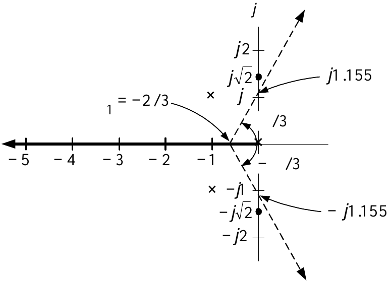
(6) Asymptotes The angles of the asymptotes are (\(n=3,m=0\)) \[\theta_{\ell}=\frac{\pi(2\ell+1)}{n-m},\text{ }\ell=0,1,...,n-m-1=\frac {\pi(2\ell+1)}{3-0},\text{ }\ell=0,1,2.\]
I.e., \(\theta_{0}=\pi/3,\theta_{1}=\pi,\theta_{2}=5\pi/3\) \((-\pi /3).\)
Their intercept on the real axis is\[\begin{aligned} \sigma_{1}=-\frac{a_{n-1}-b_{m-1}/b_{m}}{n-m},\text{ }n=3,m=0 & =-\frac {2-0}{3-0}\text{ as }a_{2}=2,b_{0}=1 \\ & =-2/3. \end{aligned}\]
Two of these asymptotes intersect the \(j\omega\) axis at \(\pm j(2/3)\tan (\pi/3)=\pm j1.155.\)
(7) Angles of Departure
For \(K=0\) the roots are at \(s=0,s=-1+j,\) and \(s=-1-j.\)
As \(K\) is increased slightly, the closed-loop poles will leave these roots.
The branch that starts at \(-1+j\) is slightly away from this point.
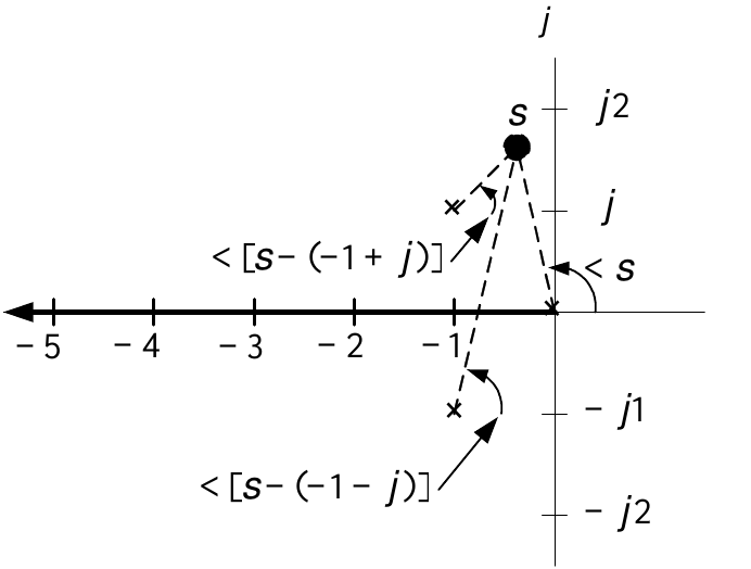
(7) Angles of Departure For \(K\) slightly positive we have\[\angle s\approx3\pi/4\text{ and }\angle\lbrack s-(-1-j)]\approx\pi/2.\]
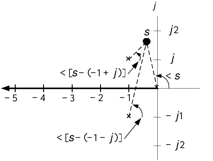
For\(s\) close to \(-1+j\) and on the root locus it must satisfy the angle condition:\[-\angle s-\underset{\text{unknown}}{\underbrace{\angle\lbrack(s-(-1+j)]}}-\angle\lbrack s-(-1-j)]=\pi(2\ell+1),\ell=0,\pm1,\pm2,....\]
Or, with \(\ell=0\), we have \(-\pi/2-\angle\lbrack(s-(-1+j)]-3\pi/4=\pi\). \[\Longrightarrow\text{ }\angle\lbrack(s-(-1+j)]=-5\pi/4-\pi=-\pi/4-2\pi =-\pi/4\text{ }\operatorname{mod}2\pi.\]
By symmetry we have \(\angle\lbrack(s-(-1-j)]=\pi/4.\)
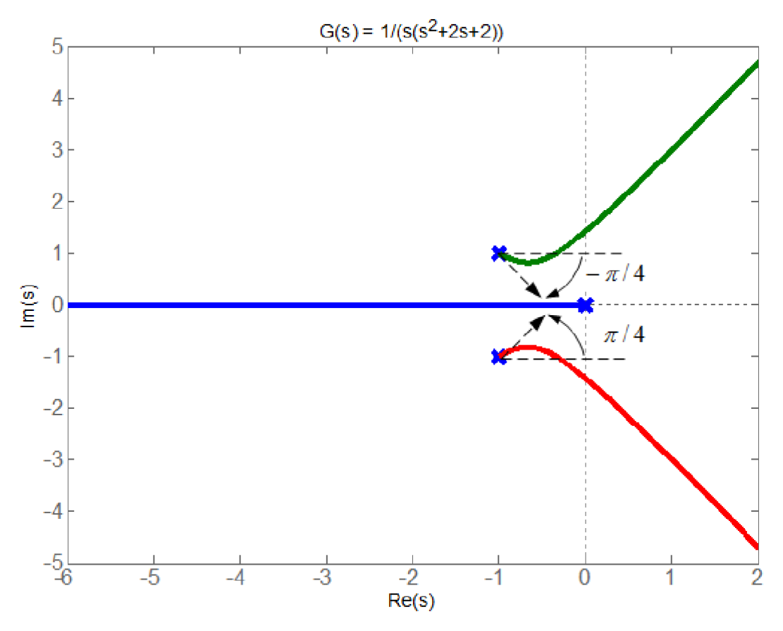
\(G(s)=\dfrac{1}{s(s^{2}+2s+2)}\)
The root locus starts on the open-loop poles.
The branch starting at \(s=0\) continues out along the negative real axis to \(-\infty.\)
The branch that starts at \(-1+j\) leaves that point at an angle of \(-\pi/4.\)
As \(K\) increases this branch intercepts the \(j\omega\) axis at \(j\sqrt{2}\).
As \(K\rightarrow\infty\) this branch approaches its asymptote.
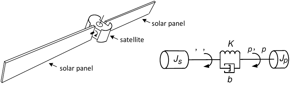
\[\begin{aligned} \theta(s) & =\frac{bs+K}{J_{s}s^{2}+bs+K}\theta_{p}(s)+\frac{1}{J_{s}s^{2}+bs+K}\tau(s) \\ \theta_{p}(s) & =\frac{bs+K}{J_{p}s^{2}+bs+K}\theta(s). \end{aligned}\]
Non collocated case: \(\theta_{p}\) is measured \[G_{p}(s)=\frac{\theta_{p}(s)}{\tau(s)}=\frac{(b/(J_{s}J_{p}))s+K/(J_{s}J_{p})}{s^{2}(s^{2}+b\left( 1/J_{p}+1/J_{s}\right) s+K\left( 1/J_{p}+1/J_{s}\right) )}.\] With \(J_{s}=5\) \(Kg-m^{2},\) \(J_{p}=1\) \(Kg-m^{2},\) \(K=0.15\) \(N-m/radian,\) \(b=0.05\) \(Nm/rad/sec,\) \(|\tau|\leq5,\) \[G_{p}(s)=\frac{0.01(s+3)}{s^{2}+0.06s+0.18}\frac{1}{s^{2}}.\]

Notch Filter \[G_{notch}(s)\triangleq\frac{s^{2}+0.06s+0.18}{(s+3)^{2}}.\] Then \[G_{notch}(s)G_{p}(s)\triangleq\frac{s^{2}+0.06s+0.18}{(s+3)^{2}}\frac{0.01(s+3)}{s^{2}+0.06s+0.18}\frac{1}{s^{2}}=\frac{0.01(s+3)}{(s+3)^{2}}\frac{1}{s^{2}}=\frac{0.01}{(s+3)s^{2}}.\]
\(G_{notch}(s)\) is used to cancel the two lightly-damped poles of \(G_{p}(s)\) at \(-0.03\pm j0.42\).
Replace them with two real poles at \(-3.\)
The location \(-3\) was chosen simply to cancel the zero of \(G_{p}(s).\)
\(G_{p}(s)\) is not known precisely so these stable pole-zero cancellations are not exact.

\[G_{notch}(s)G_{p}(s)\triangleq\frac{s^{2}+0.06s+0.18}{(s+3)^{2}}\frac{0.01(s+3)}{s^{2}+0.06s+0.18}\frac{1}{s^{2}}=\frac{0.01}{(s+3)s^{2}}.\]
A lead compensator of the form \(G_{lead}(s)=\dfrac{s+0.1}{s+1}\) stabilizes \(\dfrac{1}{s^{2}}.\)
Try this lead commpensator to stabilize \(G_{notch}(s)G_{p}(s)=\dfrac{0.01}{(s+3)s^{2}}.\)
The proposed controller is then \[G_{c}(s)=\dfrac{s+0.1}{s+1}\frac{s^{2}+0.06s+0.18}{(s+3)^{2}}.\]

\[G_{c}(s)=\dfrac{s+0.1}{s+1}\frac{s^{2}+0.06s+0.18}{(s+3)^{2}}.\]
First must deal with the fact that the cancellation is not exact.
Modify the notch filter to be \[G_{notch}(s)=\frac{s^{2}+g(0.06)s+g(0.18)}{(s+3.3)^{2}}.\]
Nominal value of \(g\) is \(1.\)
Put the poles of \(G_{notch}(s)\) at \(-3.3\) to be a little further in the left half-plane.
Consider \(g=0.8\) and \(g=1.2\) to see the effect of \(g.\)
Take \(g=0.8\) so \(G_{c}(s)=\dfrac{s+0.1}{s+1}\dfrac{s^{2}+0.048s+0.144}{(s+3.3)^{2}}.\)
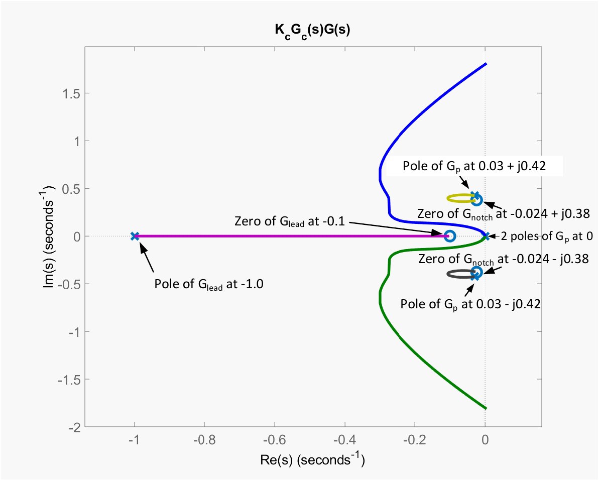
Root locus of \(K_{c}G_{c}(s)G_{p}(s)\) for \(0\leq K_{c}\leq1500.\)
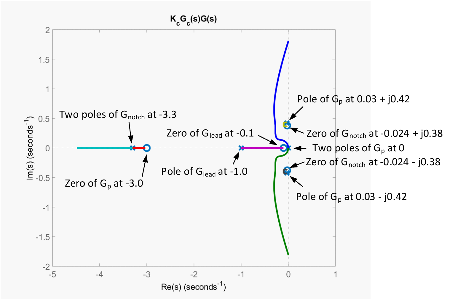
Take \(g=0.8\) so \(G_{c}(s)=\dfrac{s+0.1}{s+1}\dfrac{s^{2}+0.048s+0.144}{(s+3.3)^{2}}.\)
The 2 CL poles which start at \(-0.03\pm j0.42\) (OL poles of \(G_{p}(s)\)).
migrate to the zeros of the notch filter at \(-0.024+j0.38.\)
As \(K_{c}\) increases, they stay in the left half-plane.
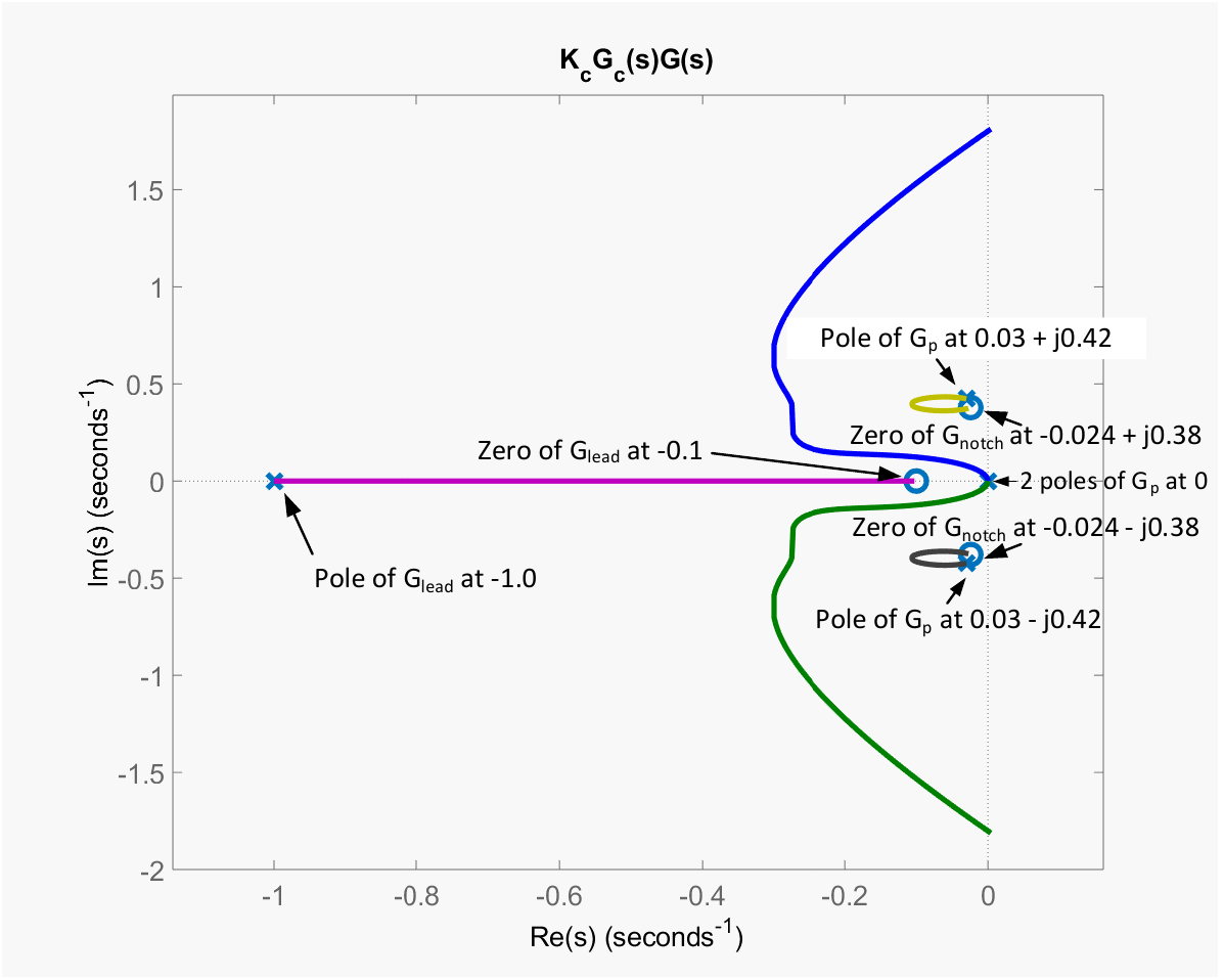
With \(K_{c}=50\) and \(g=0.8\) the closed–loop poles are at \[3.46,-3.19,-0.82,-0.044\pm j0.43,-0.054\pm j0.1.\]
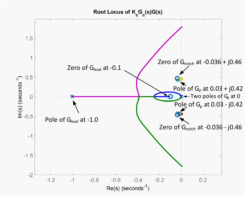
Redo root locus with \(g=1.2.\) \(G_{c}(s)=\dfrac{s+0.1}{s+1}\dfrac{s^{2}+0.072s+0.216}{(s+3.3)^{2}}.\)
The zeros of \(G_{notch}\) are now \(-0.036\pm j0.46.\)
The 2 CL poles which start at \(-0.03\pm j0.42\) (OL poles of \(G_{p}(s)\)).
migrate to the zeros of the notch filter at \(-0.036+j0.46.\)
As \(K_{c}\) increases two poles cross into the RHP!
Set \(g=0.8,\) \(K_{c}=50.\)
CL poles at \(3.46,-3.19,-0.82,-0.044\pm j0.43,-0.054\pm j0.1.\)
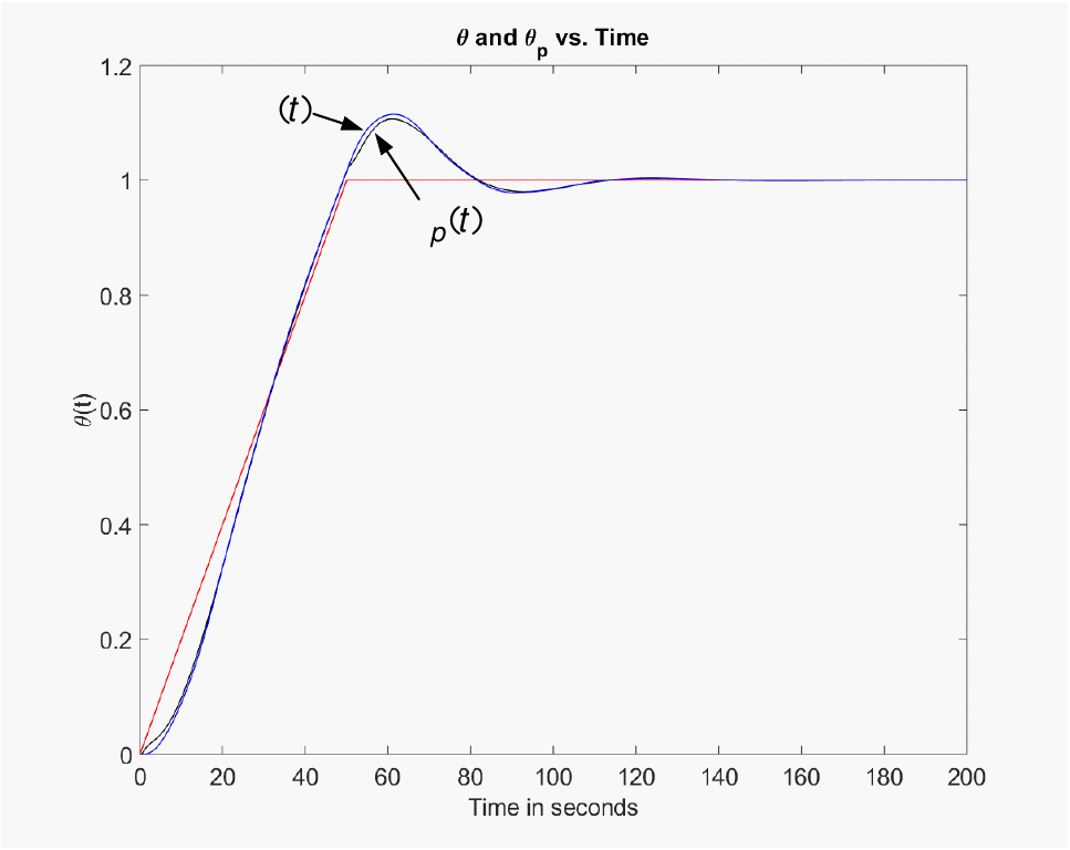
Plot of \(\theta_{p}(t)\) and \(\theta(t)\) along with \(r(t)\).
The difference \(|\theta _{p}(t)-\theta (t)|\) is small and \(|\tau (t)|<0.1.\)