Frequency Response Methods
System Modeling and Control · Chapter 11
Magnitude plot: \(20\log _{10}|G(j\omega )|\) versus \(\log _{10}\omega\)
This plot is a semilog graph, i.e., the horizontal axis is \(\log _{10}(\omega )\).
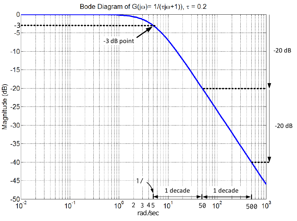
\(G(j\omega )=\dfrac{1}{\tau j\omega +1}\)
\[20\log _{10}|G(j\omega )|\;\approx \left\{ \begin{array}{cl} 0 & \;\text{for}\;\omega <1/\tau \\ -20\log _{10}\!\left( \dfrac{\omega }{1/\tau }\right) & \;\text{for}\;\omega >1/\tau .\end{array}\right.\]
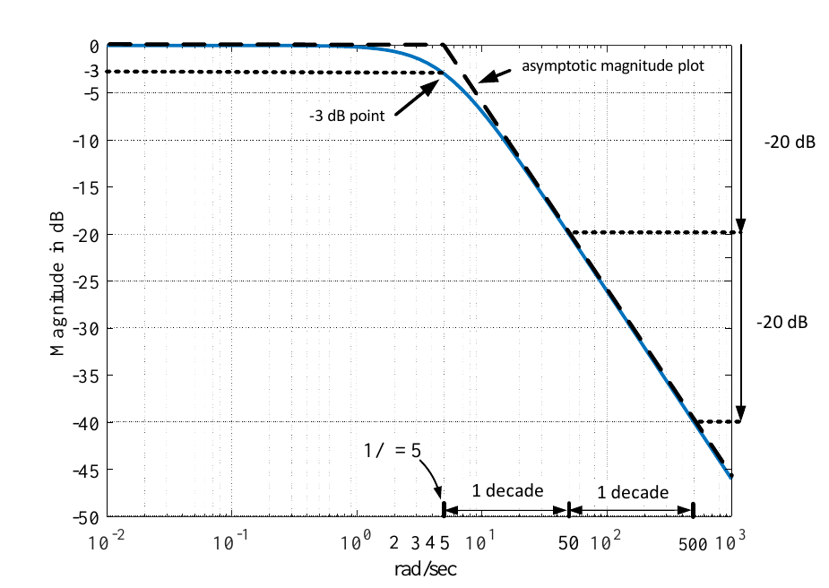
\(G(j\omega )=\dfrac{1}{\tau j\omega +1}\)
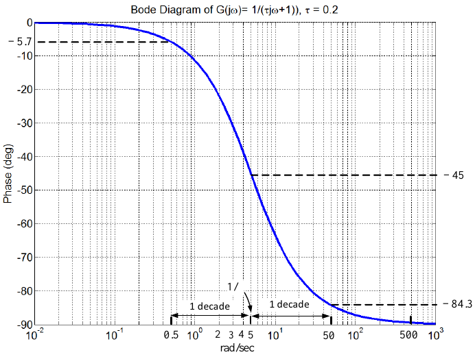
Plot \(\angle G(j\omega )\) versus \(\log _{10}\omega\).
\[\begin{array}{|l|l|l|} \hline \omega & \log _{10}(\omega ) & \angle G(j\omega )=\angle \dfrac{1}{\tau j\omega +1}=-\tan ^{-1}\!\left( \dfrac{\omega }{1/\tau }\right) \\ \hline 0 & -\infty & -\tan ^{-1}(0)=0^{\circ } \\ \hline (0.1)(1/\tau ) & -1+\log _{10}(1/\tau ) & -\tan ^{-1}(0.1)\approx -5.7^{\circ } \\ \hline 1/\tau & \log _{10}(1/\tau ) & -\tan ^{-1}(1)=-45^{\circ } \\ \hline 10(1/\tau ) & 1+\log _{10}(1/\tau ) & -\tan ^{-1}(10)=-84.3^{\circ } \\ \hline 100(1/\tau ) & 2+\log _{10}(1/\tau ) & -\tan ^{-1}(100)\approx -90^{\circ } \\ \hline \end{array}\]
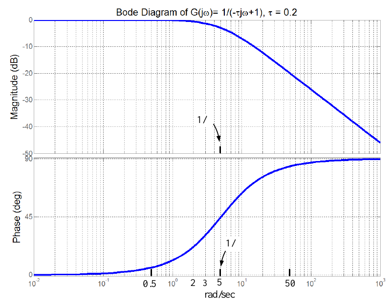
\(G(j\omega )=\dfrac{1}{-\tau j\omega +1}\)
with \(\tau =0.2\) so \(1/\tau =5\).
\[\begin{aligned} \left\vert G(j\omega )\right\vert &=&\left\vert \frac{1}{-\tau j\omega +1}\right\vert =\frac{1}{\sqrt{(\tau \omega )^{2}+1}} \\ \angle G(j\omega ) &=&\angle \dfrac{1}{-\tau j\omega +1}=-\tan ^{-1}\!\left( -\dfrac{\omega }{1/\tau }\right) =\tan ^{-1}\!\left( \dfrac{\omega }{1/\tau }\right) \end{aligned}\]
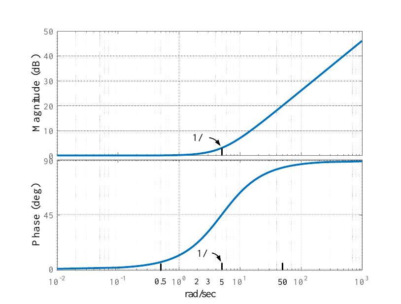
\(G(j\omega )=\tau j\omega +1\)
with \(\tau =0.2\) so \(1/\tau =5\).
\[\begin{aligned} 20\log _{10}\left\vert G(j\omega )\right\vert &=&20\log _{10}\left\vert \tau j\omega +1\right\vert =20\log _{10}\!\left\vert \sqrt{(\tau \omega )^{2}+1}\right\vert =-20\log _{10}\!\frac{1}{\sqrt{(\tau \omega )^{2}+1}} \\ \angle G(j\omega ) &=&\angle \left( \tau j\omega +1\right) =\tan ^{-1}\!\left( \dfrac{\omega }{1/\tau }\right) \end{aligned}\]
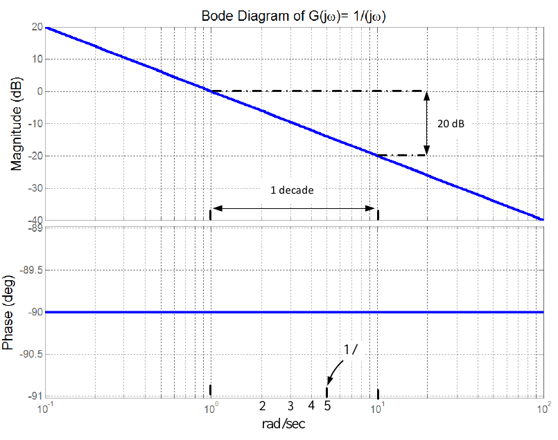
\(G(j\omega )=1/j\omega\)
\[\begin{aligned} 20\log _{10}|G(j\omega )| &=&20\log _{10}\!\left\vert 1/j\omega \right\vert =-20\log _{10}\omega \\ \angle G(j\omega ) &=&-90^{\circ }. \end{aligned}\]
Start at \(\omega =10^{0}=1\) as \(20\log _{10}|G(j1)|=-20\log _{10}\left\vert 1\right\vert =0.\)
Go to \(\omega =10\) as \(20\log _{10}|G(j\omega )|=-20\log _{10}\left\vert 10\right\vert =-20.\)
Then just draw a straight line going through these two points.
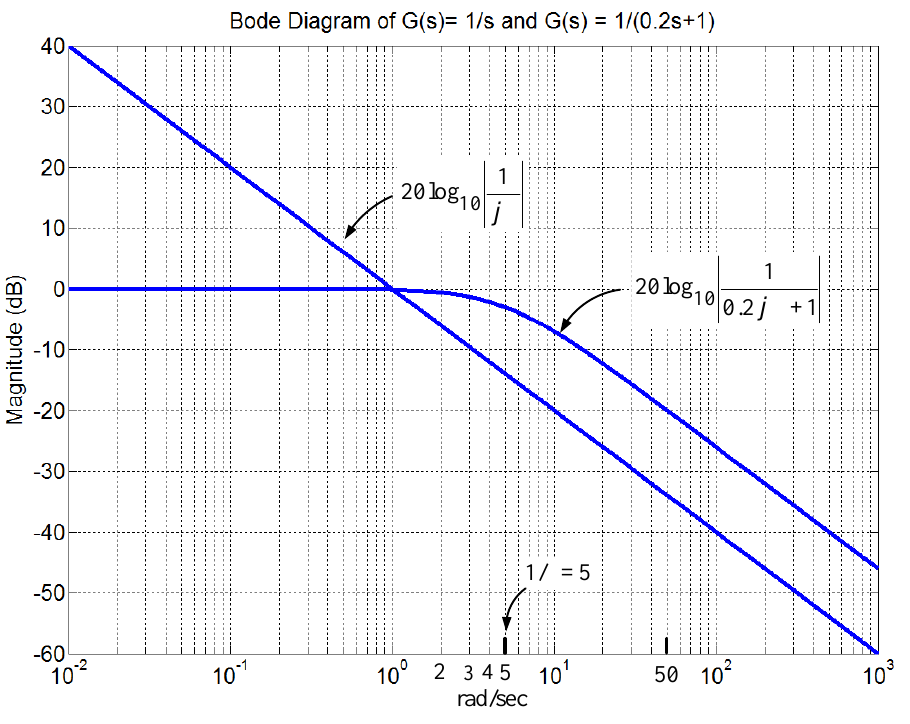
\(G(j\omega )=\dfrac{1}{j\omega (j\omega +5)}=\dfrac{1}{5}\dfrac{1}{j\omega (j\omega /5+1)},\)
\(\tau =1/5=0.2\)
\[20\log _{10}\!\left\vert \frac{1}{5}\frac{1}{j\omega (0.2j\omega +1)}\right\vert =20\log _{10}\!\left\vert \frac{1}{5}\right\vert +20\log _{10}\!\left\vert \frac{1}{j\omega }\right\vert +20\log _{10}\!\left\vert \frac{1}{j\omega /5+1}\right\vert .\]
\(G(j\omega )=\dfrac{1}{j\omega (j\omega +5)}=\dfrac{1}{5}\dfrac{1}{j\omega (j\omega /5+1)},\ \ \tau =1/5=0.2\)
First do the Bode plot of \(-20\log _{10}\left\vert \dfrac{1}{j\omega }\right\vert -20\log _{10}\left\vert \dfrac{1}{j\omega /5+1}\right\vert .\)
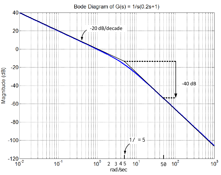
\(G(j\omega )=\dfrac{1}{j\omega (j\omega +5)}=\dfrac{1}{5}\dfrac{1}{j\omega (j\omega /5+1)},\ \ \tau =1/5=0.2\)
Finish the plot by simply adding the constant term \(20\log _{10}\!\left\vert 1/5\right\vert =-14\) dB.
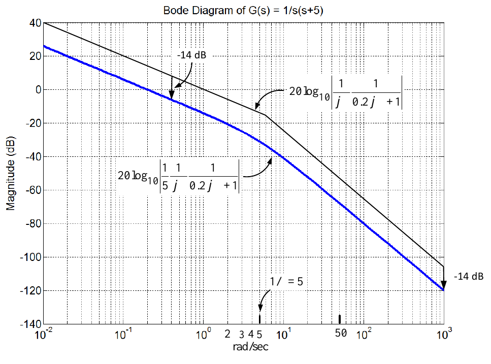
\(G(j\omega )=\dfrac{1}{j\omega (j\omega +5)}=\dfrac{1}{5}\dfrac{1}{j\omega (j\omega /5+1)},\ \ \tau =1/5=0.2\)
\[\angle \frac{1}{5}\dfrac{1}{j\omega (j\omega /5+1)}=\angle \frac{1}{5}+\angle \dfrac{1}{j\omega }+\angle \dfrac{1}{j\omega /5+1}=0^{\circ }-90^{\circ }+\angle \dfrac{1}{j\omega /5+1}.\]
At \(\omega =\dfrac{1}{10}\dfrac{1}{\tau }\) we have \(\angle G(j\omega )=-90^{\circ }-5.7^{\circ }=-95.7^{\circ }.\)
At the break point \(1/\tau =5\) we have \(\angle G(j\omega )=-90^{\circ }-45^{\circ }=-135^{\circ }.\)
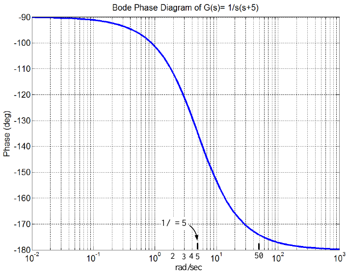
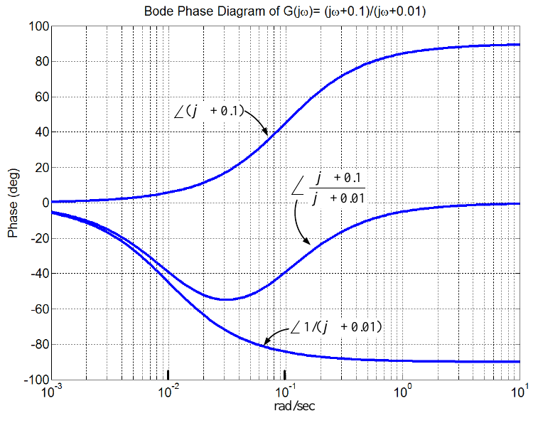
\(G_{c}(j\omega )=\dfrac{j\omega +0.1}{j\omega +0.01}\)
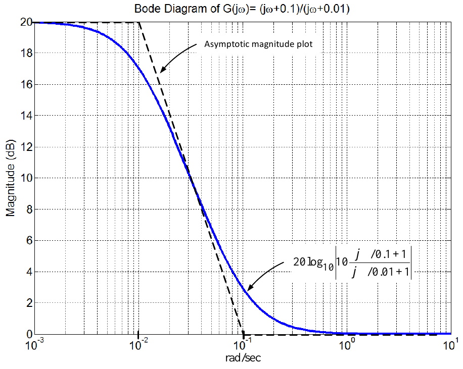
\(\angle G_{c}(j\omega )=\angle (j\omega /0.1+1)+\angle \dfrac{1}{j\omega /0.01+1}\)
\[\begin{array}{llll} \omega & \angle (j\omega /0.1+1) & \angle 1/(j\omega /0.01+1) & \angle (j\omega /0.1+1)+\angle \dfrac{1}{j\omega /0.01+1} \\ 0.001 & \approx 0 & \approx -5.7^{\circ } & \approx -5.7^{\circ } \\ 0.01 & \approx 5.7^{\circ } & \approx -45^{\circ } & \approx -39.3^{\circ } \\ 0.1 & \approx 45^{\circ } & \approx -90^{\circ } & \approx -45^{\circ } \\ 1 & \approx 90^{\circ } & \approx -90^{\circ } & \approx 0^{\circ }\end{array}\]
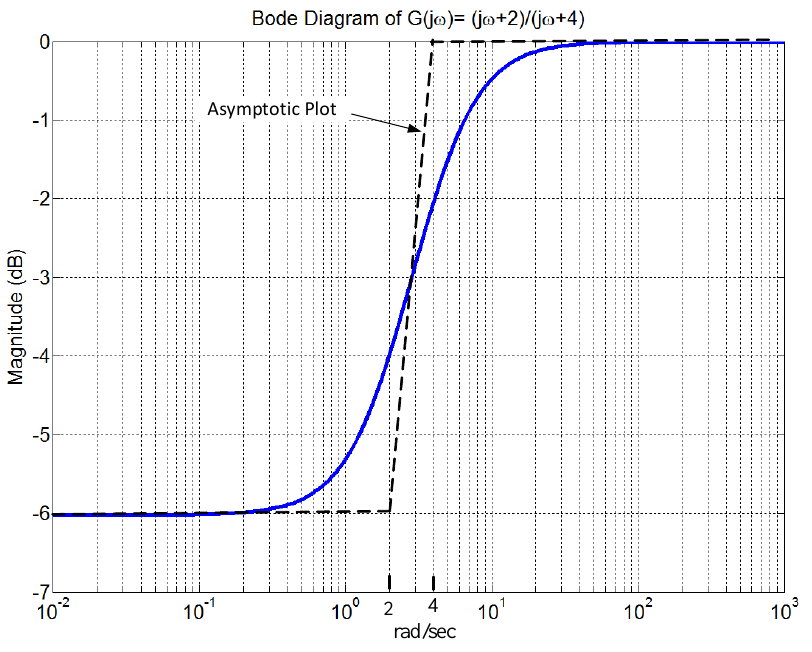
\[20\log _{10}\left\vert \dfrac{1}{2}\dfrac{j\omega /2+1}{j\omega /4+1}\right\vert =\left\{ \begin{array}{ll} 20\log _{10}|1/2|, & \omega <2 \\ 20\log _{10}|1/2|+20\log _{10}\left( \omega /2\right) , & 2<\omega <4 \\ \underset{0}{\underbrace{20\log _{10}|1/2|+20\log _{10}\left( \omega /2\right) -20\log _{10}\left( \omega /4\right) }}, & \omega >4\end{array}\right.\]
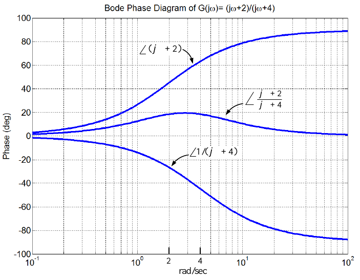
\(\ \angle G_{c}(j\omega )=\angle \dfrac{j\omega +2}{j\omega +4}=\angle (j\omega /2+1)+\angle \dfrac{1}{j\omega /4+1}\)
\[\begin{array}{lllll} \omega & & \angle (j\omega /2+1) & \angle (j\omega /4+1) & \angle (j\omega /2+1)+\angle \dfrac{1}{j\omega /4+1} \\ 0.2 & & 5.7^{\circ } & 0 & 5.7^{\circ } \\ 2 & & 45^{\circ } & \tan ^{-1}(1/2)=26.6^{\circ } & 18.4^{\circ } \\ 4 & & \tan ^{-1}(2)=63.2^{\circ } & 45^{\circ } & 18.2 \\ 20 & & 84.3^{\circ } & \tan ^{-1}(5)=78.7^{\circ } & 5.6^{\circ } \\ 40 & & 90^{\circ } & 84.3^{\circ } & 5.7^{\circ } \\ \infty & & 90^{\circ } & 90^{\circ } & 0^{\circ }\end{array}\]
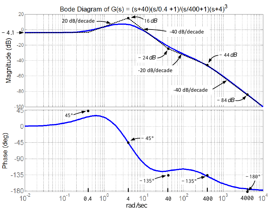
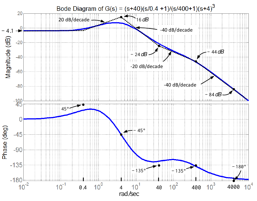
\(\ \) \(G(j\omega )=\dfrac{(j\omega +40)(j\omega /0.4+1)}{(j\omega /400+1)(j\omega +4)^{3}}=\dfrac{40}{4^{3}}\dfrac{(j\omega /40+1)(j\omega /0.4+1)}{(j\omega /400+1)(j\omega /4+1)^{3}}.\)
\[\begin{aligned} 20\log _{10}|G(j\omega )| &=&20\log _{10}\left\vert 40/64\right\vert +20\log _{10}|j\omega /0.4+1|+60\log _{10}|1/(j\omega /4+1)| \\ &&+20\log _{10}|j\omega /40+1|+20\log _{10}|1/(j\omega /400+1)| \end{aligned}\]
\(\ \)
\[\begin{array}{|c|r|r|r|r|r|r|} \hline \omega & 0.04 & 0.4 \ & 4\quad & 40\quad & 400 \ \ & 4000 \\ \hline \angle G(j\omega ) & 0^{\circ } \ & 45^{\circ } & -45^{\circ } & -135^{\circ } & -135^{\circ } & -180^{\circ } \\ \hline \end{array}\]
\(G(s)=\dfrac{\omega _{n}^{2}}{s^{2}+2\zeta \omega _{n}s+\omega _{n}^{2}}\)
\(0<\zeta <1\)
\[20\log _{10}\left\vert \frac{1}{(j\omega /\omega _{n})^{2}}\right\vert =\left\{ \begin{array}{ll} 0, & \omega <\omega _{n} \\ 20\log _{10}\left\vert \dfrac{1}{(j\omega /\omega _{n})^{2}}\right\vert =-40\log _{10}\left\vert \omega /\omega _{n}\right\vert , & \omega >\omega _{n}.\end{array}\right.\]
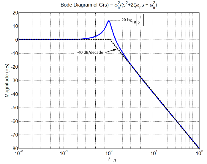
\(\omega _{n}\) is a (double) breakpoint.
The asymptotic magnitude plot decreases at \(-40\) dB/decade after the breakpoint.
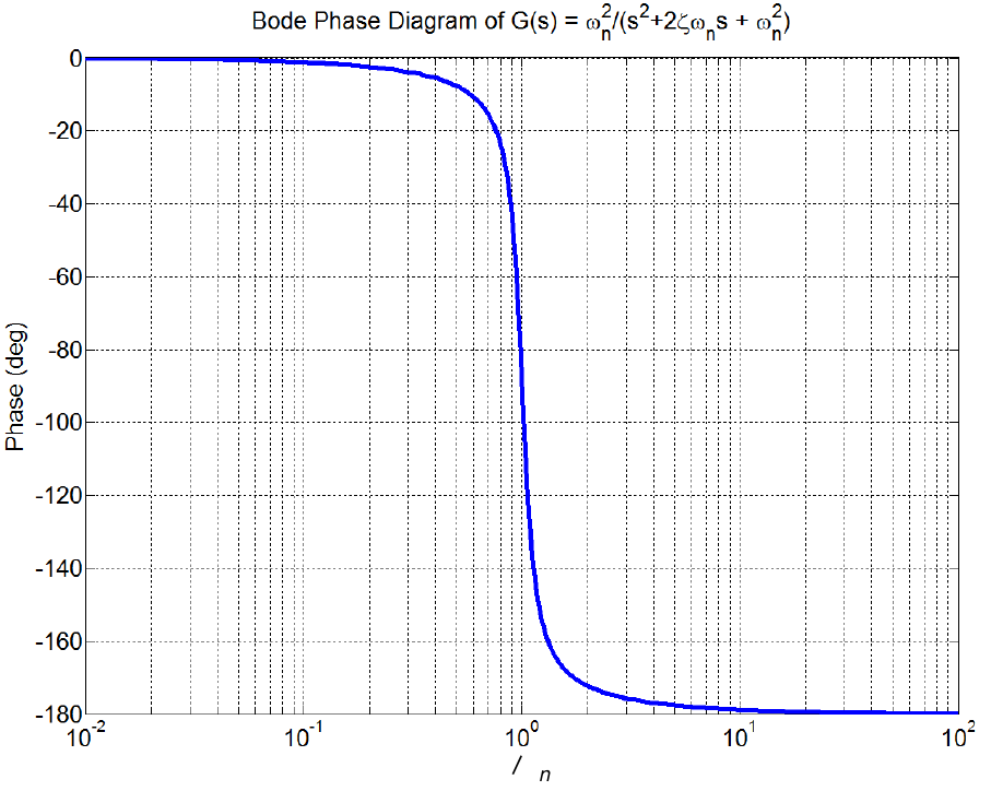
\(G(s)=\omega _{n}^{2}/(s^{2}+2\zeta \omega _{n}s+\omega ^{2})\)
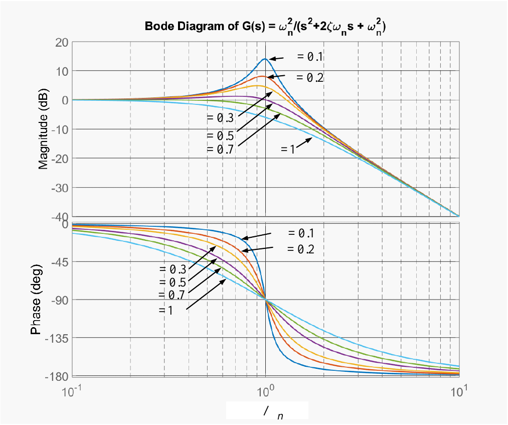
\[\angle G(j\omega )=\angle \dfrac{1}{(j\omega /\omega _{n})^{2}+2\zeta j\omega /\omega _{n}+1}=-\tan ^{-1}\!\left( \frac{2\zeta (\omega /\omega _{n})}{1-(\omega /\omega _{n})^{2}}\right) .\]
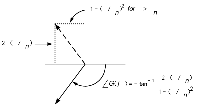
\[\begin{array}{|l|l|l|} \hline \omega & \log _{10}\omega & \angle G(j\omega )=-\tan ^{-1}\!\left( \dfrac{2\zeta (\omega /\omega _{n})}{1-(\omega /\omega _{n})^{2}}\right) \\ \hline 0 & -\infty & 0 \\ \hline 0.1\omega _{n} & -1+\log _{10}\omega _{n} & -\tan ^{-1}\!\left( \dfrac{2\zeta /10}{1-1/100}\right) \approx -\tan ^{-1}(\zeta /5) \\ \hline \omega _{n} & \log _{10}\omega _{n} & -\tan ^{-1}\!\left( \dfrac{2\zeta }{0}\right) =-90^{\circ } \\ \hline 10\omega _{n} & 1+\log _{10}\omega _{n} & -\tan ^{-1}\!\left( \dfrac{20\zeta }{1-100}\right) \approx -180^{\circ }+\tan ^{-1}(\zeta /5) \\ \hline \infty & \infty & -180^{\circ } \\ \hline \end{array}\]
The phase plot where \(\omega _{n}=1\) and \(\zeta =0.1.\)
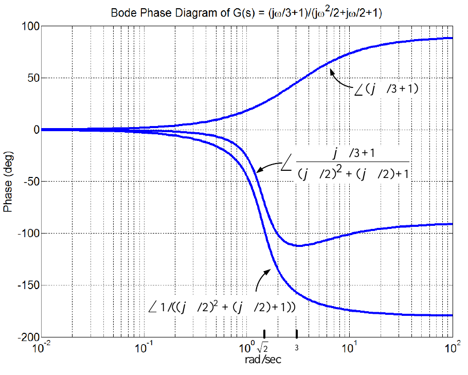
\(G(j\omega )=\dfrac{j\omega /3+1}{(j\omega )^{2}/2+j\omega /2+1}=\dfrac{j\omega /3+1}{(j\omega /\omega _{n})^{2}+2\zeta j\omega /\omega _{n}+1}\) \(\Longrightarrow \omega _{n}^{2}=2,\)
\(2\zeta /\omega _{n}=1/2\) or \(\omega _{n}=\sqrt{2},\ \ \zeta =1/(2\sqrt{2})=0.35.\)
For \(\omega >\sqrt{2}\) the magnitude \(\downarrow\) at \(-40\) dB/decade.
For \(\omega >3\) after breakpoint of the zero, magnitude \(\downarrow\) at only \(-20\) dB/decade.
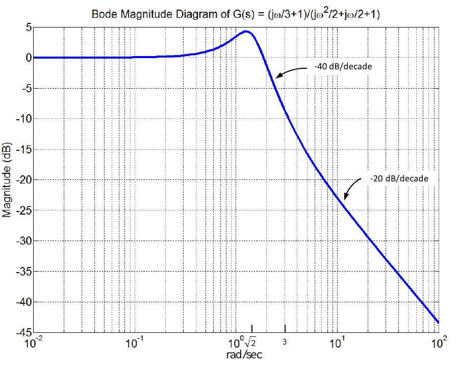
\(G(j\omega )=\dfrac{j\omega /3+1}{(j\omega )^{2}/2+j\omega /2+1}\)
- Gives a method to determine stability from the open-loop Bode diagram.
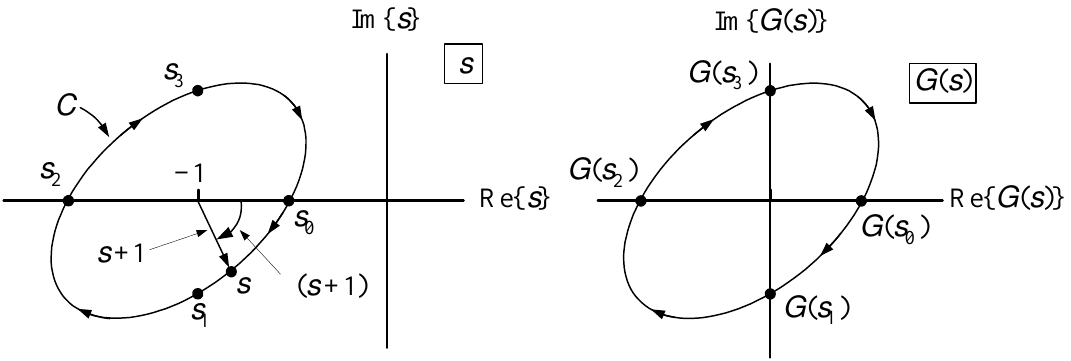
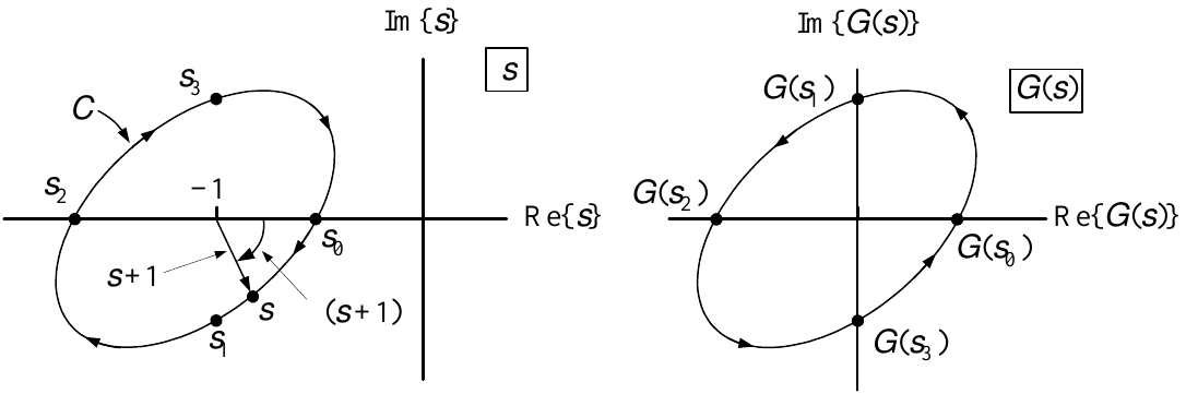
Principle of the Argument Let
\[G(s)=s+1=s-(-1)=|s+1|e^{j\angle (s+1)}.\]
Let “\(s\)” go around \(\mathcal{C}\) once in the clockwise direction.
“\(s\)” successively goes through \(s_{0},s_{1},s_{2},s_{3}\) and back to \(s_{0}.\)
\(\angle G(s_{i})=\angle (s_{i}+1)=0,-\pi /2,-\pi ,-3\pi /2,-2\pi ,\) respectively.
I.e., the image \(G(s)\) goes around the origin once in the clockwise direction.
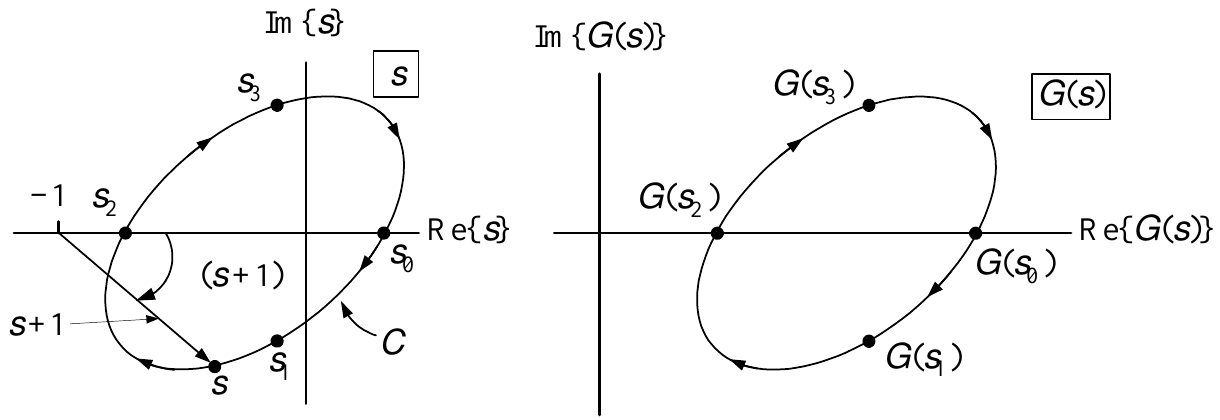
Let
\[G(s)=\frac{1}{s+1}=\frac{1}{|s+1|}e^{-j\angle (s+1)}\]
Let “\(s\)” go around \(\mathcal{C}\) once in the clockwise direction.
“\(s\)” successively goes through \(s_{0},s_{1},s_{2},s_{3}\) and back to \(s_{0}.\)
\(\angle G(s_{i})=-\angle (s_{i}+1)=0,\pi /2,\pi ,3\pi /2,2\pi ,\) respectively.
The image \(G(s)\) goes around the origin once in the counterclockwise direction.
Let
\[G(s)=s+1=s-(-1)=|s+1|e^{j\angle (s+1)}\]
The zero at \(s=-1\) is not inside the curve \(\mathcal{C}\).
Let “\(s\)” travel around closed curve \(\mathcal{C}\) once in the counterclockwise direction.
“\(s\)” successively goes through \(s_{0},s_{1},s_{2},s_{3}\) and back to \(s_{0}\).
The image \(G(s)\) does not go around the origin.
This is because \(\angle (s+1)\) does not change by \(2\pi\) as we go around \(\mathcal{C}\).
\[\begin{aligned} G(s)=\frac{(s-z_{1})(s-z_{2})}{(s-p_{1})(s-p_{2})} &=&\frac{|s-z_{1}|e^{j\angle (s-z_{1})}|s-z_{2}|e^{j\angle (s-z_{2})}}{|s-p_{1}|e^{j\angle (s-p_{1})}|s-p_{2}|e^{j\angle (s-p_{2})}} \\ &=&\frac{|s-z_{1}||s-z_{2}|}{|s-p_{1}||s-p_{2}|}e^{j\angle (s-z_{1})}e^{j\angle (s-z_{2})}e^{-j\angle (s-p_{1})}e^{-j\angle (s-p_{2})}. \end{aligned}\]
\(z_{2}\) is outside the curve
\(z_{1},p_{1},p_{2}\) are inside the curve.
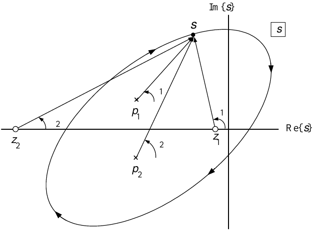
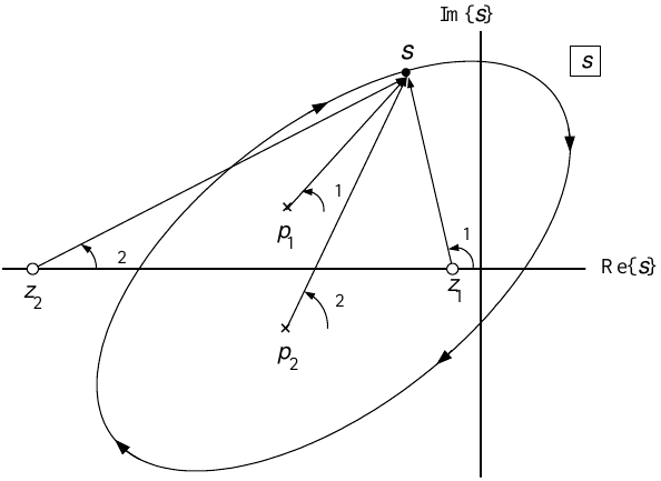
\[\begin{array}{|l|l|l|} \hline \text{Pole/Zero} & \text{Change in angle} & \;\text{Causes}\;G(s)\;\text{to go around the origin}\; \\ \hline \angle \dfrac{1}{s-p_{1}}=-\phi _{1} & +2\pi & \text{Once in the CCW direction} \\ \hline \angle \dfrac{1}{s-p_{2}}=-\phi _{2} & +2\pi & \text{Once in the CCW direction} \\ \hline \angle (s-z_{1})=\theta _{1} & -2\pi & \text{Once in the CW direction} \\ \hline \angle (s-z_{2})=\theta _{2} & \quad 0 & \text{Zero} \\ \hline \end{array}\]
As “\(s\)” goes around the closed curve once in the clockwise direction, the image \(G(s)\) goes around the origin once in the counterclockwise direction.
Principle of the Argument \(G(s)=\dfrac{1}{(s+1)(s+3)}.\)
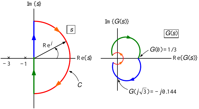
For \(\omega \geq 0\) we have
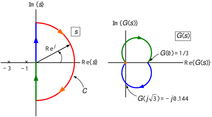
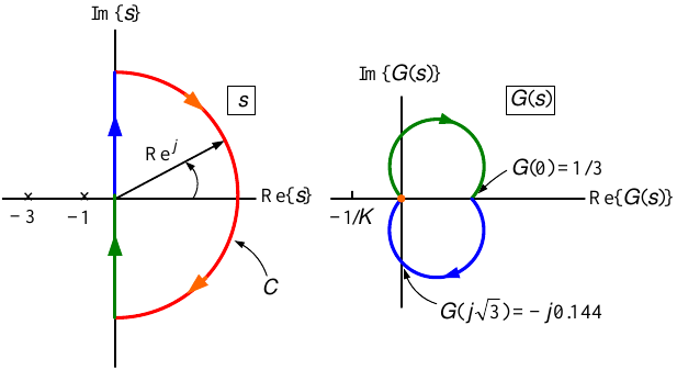
\[G(j\omega )=\frac{1}{(j\omega +1)(j\omega +3)}=\frac{(1-j\omega )(3-j\omega )}{(1+\omega ^{2})(9+\omega ^{2})}=\frac{3-\omega ^{2}-j4\omega }{(1+\omega ^{2})(9+\omega ^{2})}\]
so that
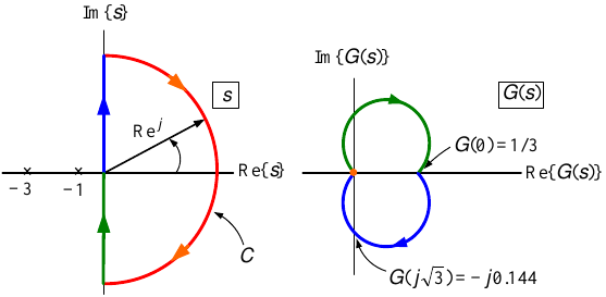
\[G(j0)=1/3,\;G(j\sqrt{3})=\frac{-j4\sqrt{3}}{(4)(12)}=-j0.144,\;G(j\omega )\approx -\frac{1}{\omega ^{2}}\;\text{for}\;\omega \;\text{large.}\;\]
Principle of the Argument \(G(s)=\dfrac{1}{(s+1)(s+3)}\) \(.\)
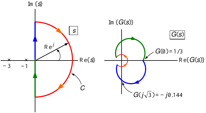
On the semicircle \(s=Re^{j\theta },\) \(-\pi /2\leq \theta \leq \pi /2\)
\[G(Re^{j\theta })=\frac{1}{(Re^{j\theta }+1)(Re^{j\theta }+3)}\approx \frac{1}{R^{2}}e^{-j2\theta }\;\text{as}\;R\;\text{is large.}\;\begin{array}{|c|l|} \hline \theta & G(Re^{j\theta })\approx e^{-j2\theta }/R^{2} \\ \hline \pi /2 & e^{-j\pi }/R^{2}=-1/R^{2} \\ \hline \pi /4 & e^{-j\pi /2}/R^{2}=-j/R^{2} \\ \hline 0 & e^{j0}/R^{2}=1/R^{2} \\ \hline -\pi /4 & e^{j\pi /2}/R^{2}=j/R^{2} \\ \hline -\pi /2 & e^{j\pi }/R^{2}=-1/R^{2} \\ \hline \end{array}\]
Principle of the Argument \(G(s)=\dfrac{1}{(s+1)(s+3)}\)
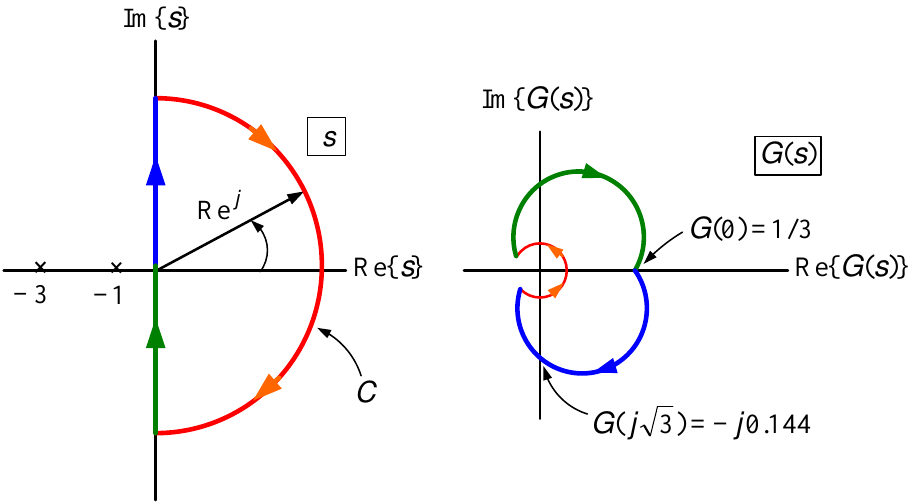
For \(\omega \leq 0\) the image \(G(j\omega )\) is simply the complex conjugate of the image for \(\omega \geq 0.\)
No poles nor zeros of \(G(s)\) inside the closed curve \(\mathcal{C}\) so \(P=Z=0.\)
By inspection the image of \(G(s)\) on \(\mathcal{C}\) does not go around the origin so \(N=0.\)
This verifies the principle of the argument, i.e.,
\[N=Z-P.\]
Principle of the Argument \(G(s)=\dfrac{1}{(s+1)(s+3)}\) Choose \(\mathcal{C}\) to enclose the left half-plane.
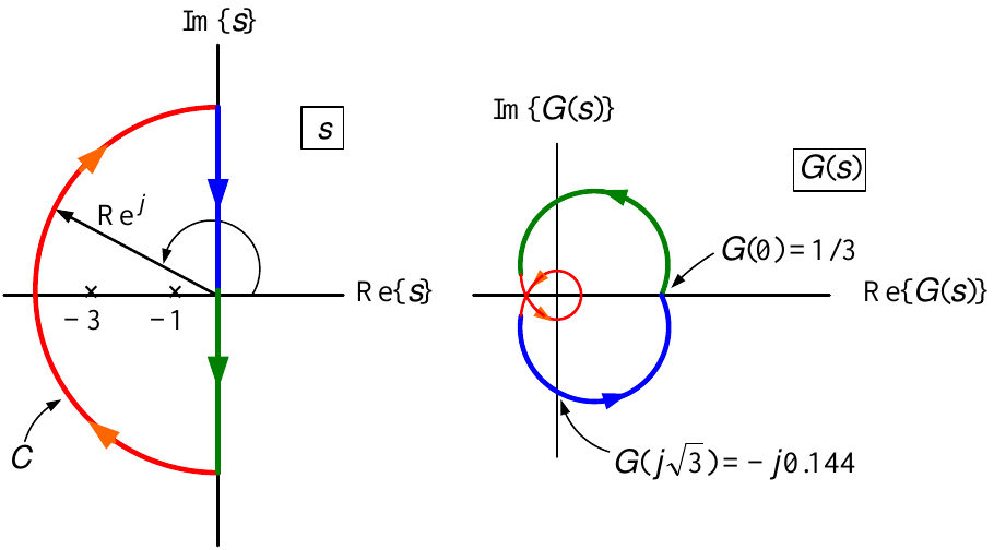
For \(-\infty <\omega <\infty\) the image \(G(j\omega )\) is the same as in the previous example.
On the semicircle \(s=Re^{j\theta },\) \(-\pi /2\leq \theta \leq -3\pi /2\)
\[G(Re^{j\theta })=\frac{1}{(Re^{j\theta }+1)(Re^{j\theta }+3)}\approx \frac{1}{R^{2}}e^{-j2\theta }\;\text{as}\;R\;\text{is large.}\;\]
Principle of the Argument \(G(s)=\dfrac{1}{(s+1)(s+3)}\)
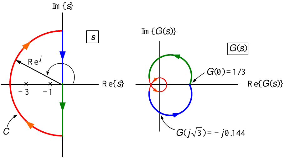
\[\begin{array}{|c|c|} \hline \theta & G(Re^{j\theta })\approx \dfrac{1}{R^{2}}e^{-j2\theta } \\ \hline -\pi /2 & e^{j\pi }/R^{2}=-1/R^{2} \\ \hline -3\pi /4 & e^{j3\pi /2}/R^{2}=-j/R^{2} \\ \hline -\pi & e^{j2\pi }/R^{2}=1/R^{2} \\ \hline -5\pi /4 & e^{j5\pi /2}/R^{2}=j/R^{2} \\ \hline -3\pi /2 & e^{j3\pi }/R^{2}=-1/R^{2} \\ \hline \end{array}\]
Principle of the Argument \(G(s)=\dfrac{1}{(s+1)(s+3)}\)
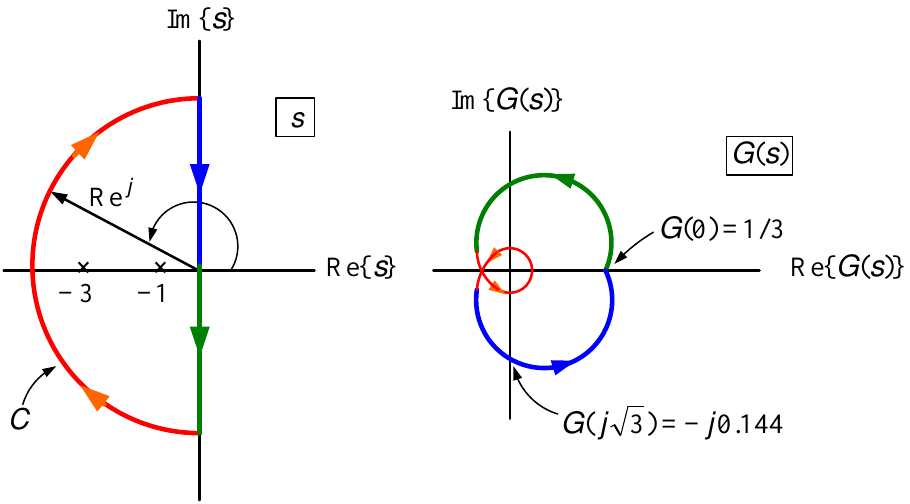
There are two poles of \(G(s)\) inside the closed curve \(\mathcal{C}\) so \(P=2.\)
There are no zeros of \(G(s)\) inside the closed curve \(\mathcal{C}\) so \(Z=0.\)
By inspection the image of \(G(s)\) on this curve goes around the origin twice
in the counterclockwise direction so \(N=-2.\)
We have thus verified that
\[N=Z-P.\]
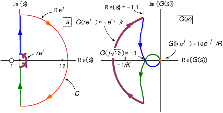
Principle of the Argument \(G(s)=\dfrac{10(s+1)}{s(s-10)}=-\dfrac{s+1}{s(-s/10+1)}\)
The closed curve \(\mathcal{C}\) is taken to enclose the right half-plane.
Let \(s=Re^{j\theta }\) with \(-\pi /2\leq \theta \leq \pi /2\) and let \(R\rightarrow \infty .\)
Avoid pole at \(s=0\) by letting \(s=re^{j\theta },\) \(-\pi /2\leq \theta \leq \pi /2\) with \(r\rightarrow 0.\)
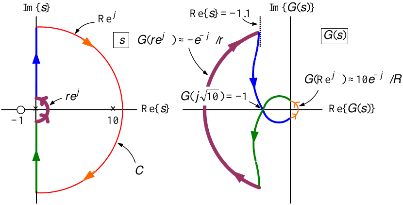
For \(s=j\omega\) we have
\[\begin{aligned} G(j\omega )=-\frac{j\omega +1}{j\omega (-j\omega /10+1)} &=&-\frac{(j\omega +1)(-j\omega )(j\omega /10+1)}{\omega ^{2}(\omega ^{2}/100+1)} \\ &=&\frac{-\omega ^{2}(1+1/10)+j\omega (1-\omega ^{2}/10)}{\omega ^{2}(\omega ^{2}/100+1)}. \end{aligned}\]
Principle of the Argument \(G(s)=\dfrac{10(s+1)}{s(s-10)}=-\dfrac{s+1}{s(-s/10+1)}\)
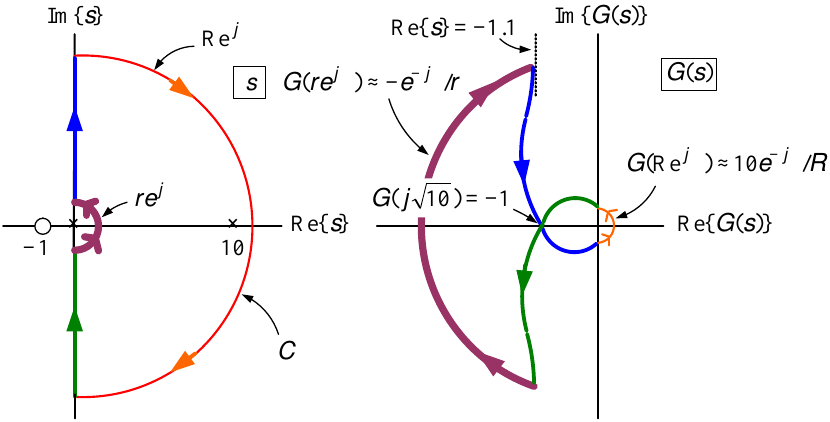
\[\begin{aligned} G(j\omega ) &=&\frac{-\omega ^{2}(1+1/10)+j\omega (1-\omega ^{2}/10)}{\omega ^{2}(\omega ^{2}/100+1)} \\ G(j\omega ) &\approx &-1.1+\frac{j}{\omega }\;\text{for}\;0<\omega <<1 \\ G(j\sqrt{10}) &=&-\frac{10(1+1/10)}{10(10/100+1)}=-1 \\ G(j\omega ) &\approx &-\frac{j10}{\omega }\;\text{for}\;\omega >>1. \end{aligned}\]
Principle of the Argument \(G(s)=\dfrac{10(s+1)}{s(s-10)}=-\dfrac{s+1}{s(-s/10+1)}\)
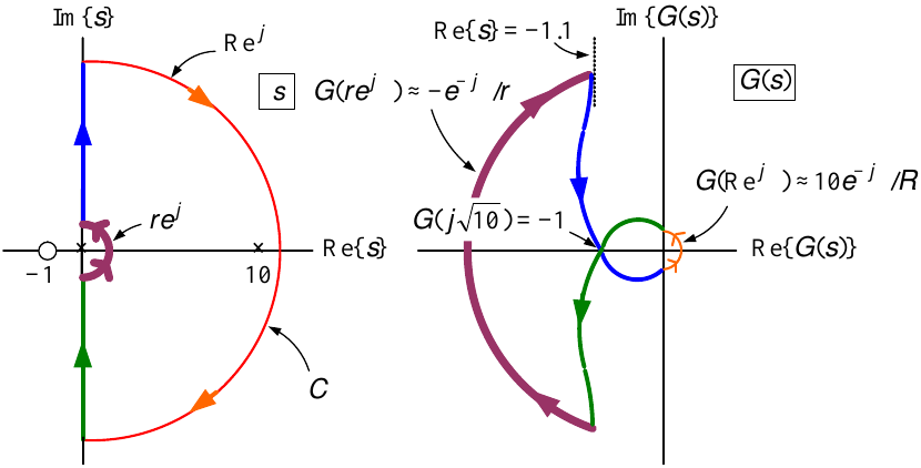
\[G(re^{j\theta })=\frac{10(re^{j\theta }+1)}{re^{j\theta }(re^{j\theta }-10)}\approx \frac{10}{re^{j\theta }(-10)}=-e^{-j\theta }/r.\begin{array}{|c|c|} \hline \ \ \theta & G(re^{j\theta })\approx -\dfrac{1}{r}e^{-j\theta } \\ \hline -\pi /2 & -e^{j\pi /2}/r=-j/r \\ \hline -\pi /4 & -e^{j\pi /4}/r \\ \hline 0 \ \ & -1/r \\ \hline \pi /4 & -e^{-j\pi /4}/r \\ \hline \pi /2 & -e^{-j\pi /2}/r=j/r \\ \hline \end{array}\]
Principle of the Argument \(G(s)=\dfrac{10(s+1)}{s(s-10)}=-\dfrac{s+1}{s(-s/10+1)}\)
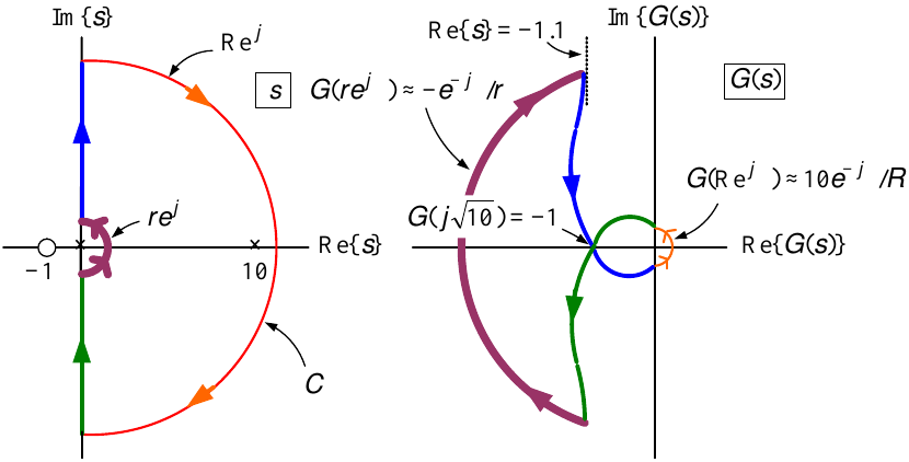
\(s=Re^{j\theta },\) \(-\pi /2\leq \theta \leq \pi /2\)
\[G(Re^{j\theta })=\frac{10(Re^{j\theta }+1)}{Re^{j\theta }(Re^{j\theta }-10)}\approx \frac{10Re^{j\theta }}{Re^{j\theta }Re^{j\theta }}=10e^{-j\theta }/R.\begin{array}{|c|c|} \hline \theta & G(Re^{j\theta })\approx \dfrac{10}{R}e^{-j\theta } \\ \hline \pi /2 & -j10/R \\ \hline 0 & \ \ \ 10/R \\ \hline \!\!\!-\pi /2 & \ \ j10/R \\ \hline \end{array}\]
Principle of the Argument \(G(s)=\dfrac{10(s+1)}{s(s-10)}=-\dfrac{s+1}{s(-s/10+1)}\)
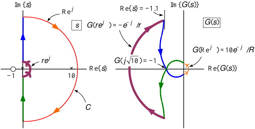
\(G(s)\) has one pole inside the closed curve \(\mathcal{C}\) so \(P=1.\)
\(G(s)\) has no zeros of \(G(s)\) inside the closed curve \(\mathcal{C}\) so \(Z=0.\)
By inspection the image of \(G(s)\) on \(\mathcal{C}\) goes around the origin once
in the counterclockwise direction. I.e., \(N=-1.\)
We have thus verified that \(N=Z-P\) as both sides equal \(-1.\)
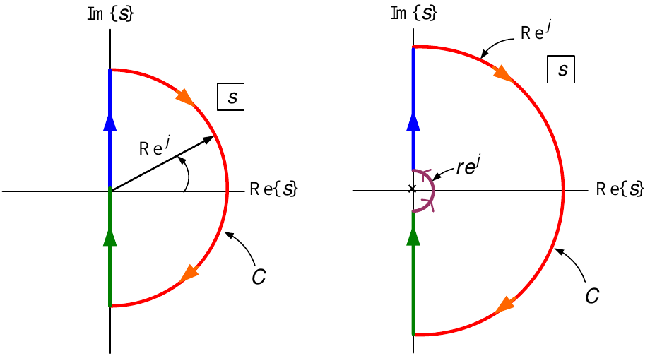
Nyquist Contour
A simple closed-curve enclosing the right half-plane.
The direction of travel is the clockwise direction.
Examples Nyquist Contour
In both examples below let \(R\rightarrow \infty .\)
An open-loop pole on the \(j\omega\) axis is bypassed using a semicircular detour with \(r\rightarrow 0.\)
Nyquist Polar Plot
The Nyquist polar plot is a plot of \(G(s)\) as \(s\) goes around the Nyquist contour in a clockwise fashion.
Example Nyquist Polar Plot \(G(s)=\dfrac{1}{(s+1)(s+3)}\)
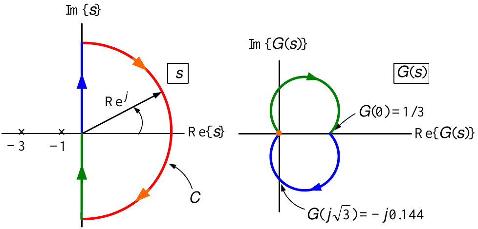
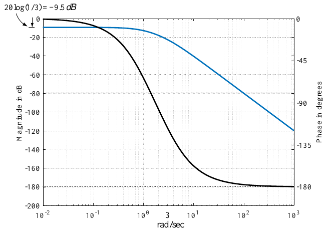
Key observation: The part of the Nyquist polar plot due to the \(j\omega\) axis is found from the Bode diagram of \(G(j\omega )\).
\(G(j\omega )=\dfrac{1}{(j\omega +1)(j\omega +3)}=\dfrac{1}{3}\dfrac{1}{(j\omega +1)(j\omega /3+1)}\)
\(G(s)=\dfrac{10(s+1)}{s(s-10)}=-\dfrac{s+1}{s(-s/10+1)}\)
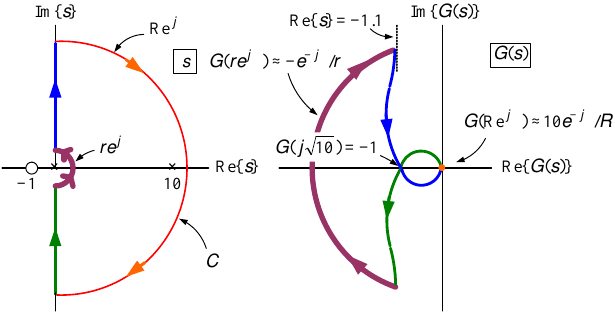
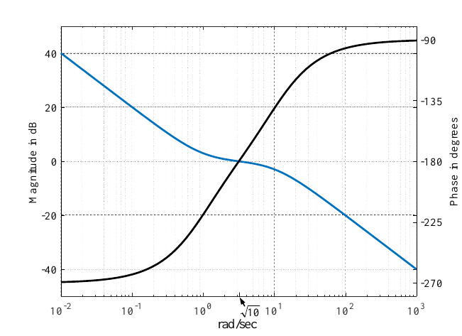
\(G(s)=\dfrac{10(s+1)}{s(s-10)}=-\dfrac{s+1}{s(-s/10+1)}\)
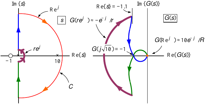
\(G(Re^{j\theta })=\dfrac{10(Re^{j\theta }+1)}{Re^{j\theta }(Re^{j\theta }-10)}\approx \dfrac{10Re^{j\theta }}{Re^{j\theta }Re^{j\theta }}=\dfrac{10e^{-j\theta }}{R}\rightarrow 0\) as \(R\rightarrow \infty .\)
\(G(re^{j\theta })=\dfrac{10(re^{j\theta }+1)}{re^{j\theta }(re^{j\theta }-10)}\approx \dfrac{10}{re^{j\theta }(-10)}=-\dfrac{e^{-j\theta }}{r}\)
where \(-\pi /2\leq \theta \leq \pi /2\) and \(r\rightarrow 0.\)
Open-loop transfer function: \(G(s)=\dfrac{1}{(s+1)(s+3)}\)
Proportional controller:
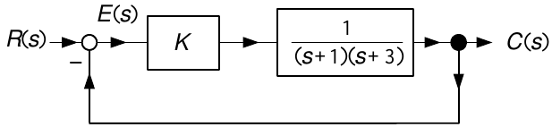
Closed-loop transfer function:
\[\frac{C(s)}{R(s)}=\frac{KG(s)}{1+KG(s)}=\frac{\dfrac{K}{(s+1)(s+3)}}{1+\dfrac{K}{(s+1)(s+3)}}=\frac{K}{(s+1)(s+3)+K}.\]
Closed-loop poles are the zeros of the Return Difference:
\[1+KG(s)=1+\dfrac{K}{(s+1)(s+3)}=\frac{(s+1)(s+3)+K}{(s+1)(s+3)}=0\]
Closed-loop system is stable if and only if
\[1+KG(s)\neq 0\;\text{for}\;\operatorname{Re}\{s\}\geq 0\]
or equivalently,
\[\frac{1}{K}+G(s)\neq 0\;\text{for}\;\operatorname{Re}\{s\}\geq 0.\]
\(1+KG(s)=1+\dfrac{K}{(s+1)(s+3)}=\dfrac{(s+1)(s+3)+K}{(s+1)(s+3)}=0\)
Nyquist stability test: Apply the principle of the argument to
\[\frac{1}{K}+G(s).\]
The curve \(\mathcal{C}\) encloses the right half-plane.
Draw the corresponding polar plot.
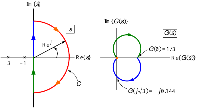
With \(K>0\) shift the polar plot to the right by \(1/K\).
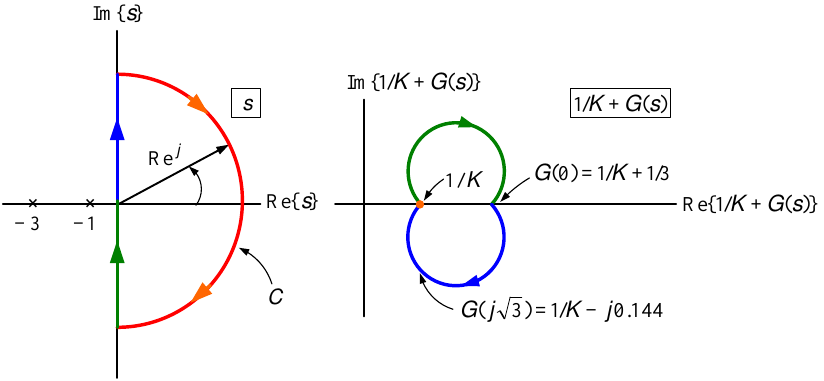
\(\dfrac{1}{K}+G(s)=\dfrac{1}{K}\dfrac{(s+1)(s+3)+K}{(s+1)(s+3)}\)
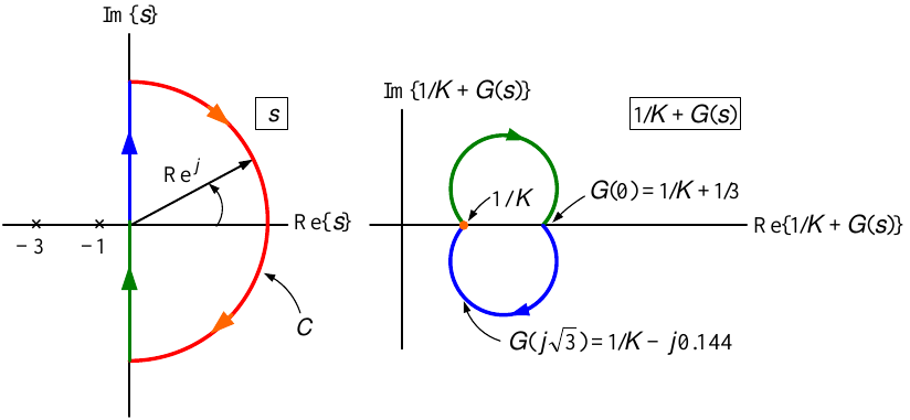
The poles of \(1/K+G(s)\) are the poles of \(G(s)\).
These are not inside the curve \(\mathcal{C}\) so \(P=0.\)
With \(K>0\) the image of \(1/K+G(s)\) does not go around the origin so \(N=0.\)
By the principle of the argument we have
\[N=Z-P\]
or
\[Z=N+P=0+0=0.\]
So \(1/K+G(s)\) has no roots in the RHP \(\Longrightarrow\) closed-loop system is stable.
\(\dfrac{1}{K}+G(s)=\dfrac{1}{K}\left( 1+KG(s)\!\right) =\dfrac{1}{K}\dfrac{(s+1)(s+3)+K}{(s+1)(s+3)}\)
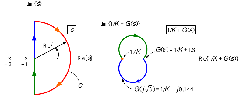
\(1/K+G(s)\) goes around the origin if and only if \(G(s)\) goes around \(-1/K.\)
Draw the Nyquist plot of \(G(s)\) and mark the \(-1/K\) point on the plot.
With \(K>0\) the polar plot of \(G(s)\) does not go around \(-1/K\) \(\Longrightarrow N=0.\)
\(G(s)=\dfrac{10(s+1)}{s(s-10)}=-\dfrac{s+1}{s(-s/10+1)}\)
\(\dfrac{1}{K}\left( 1+KG(s)\!\right) =\dfrac{1}{K}\left( 1+K\dfrac{10(s+1)}{s(s-10)}\right) =\dfrac{1}{K}\dfrac{s(s-10)+K10(s+1)}{s(s-10)}.\)
The pole of \(G(s)\) at \(s=10\) is inside the curve \(\mathcal{C}\) so \(P=1.\)
The number of times \(1/K+G(s)\) goes around the origin is the same as the number of times \(G(s)\) goes around \(-1/K.\)
Case (1) Suppose \(-\infty <-1/K<-1\) which means \(0<K<1.\)
Then \(N=1\) as \(G(s)\) goes around \(-1/K\) once in the clockwise direction. As \(N=Z-P\)
\[Z=N+P=1+1=2\]
\(1/K+G(s)=0\) has two zeros in the right half-plane.
The closed-loop system is unstable for \(0<K<1.\)
\(G(s)=\dfrac{10(s+1)}{s(s-10)}=-\dfrac{s+1}{s(-s/10+1)}\)
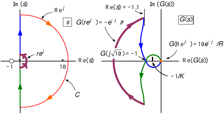
Case (2) Suppose \(-1<-1/K<0\) which means \(K>1.\)
\(N=-1\) as \(G(s)\) goes around \(-1/K\) once in the counterclockwise direction.
By the mapping theorem we have
\[Z=N+P=-1+1=0\]
\(1/K+G(s)=0\) has no zeros in the right half-plane.
The closed-loop system is stable for \(K>1.\)
Check: Apply the Routh-Hurwitz test to \(s(s-10)+10K(s+1)=0.\)
\(G(s)=\dfrac{1}{(s+1)(s^{2}+\sqrt{2}s+1)}\) \(=\dfrac{1}{(s+1)(s-[-1/\sqrt{2}+j/\sqrt{2}])(s-[-1/\sqrt{2}-j/\sqrt{2}])}\)
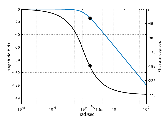
\(G(s)=\dfrac{1}{(s+1)(s^{2}+\sqrt{2}s+1)}\) \(=\dfrac{1}{(s+1)(s-[-1/\sqrt{2}+j/\sqrt{2}])(s-[-1/\sqrt{2}-j/\sqrt{2}])}\)
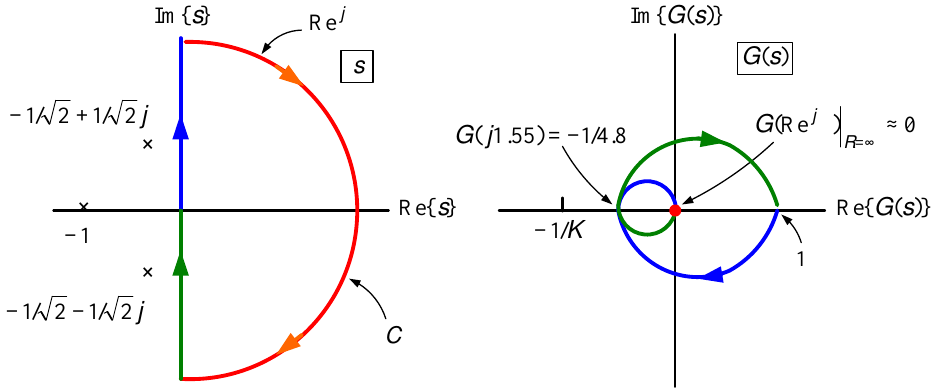
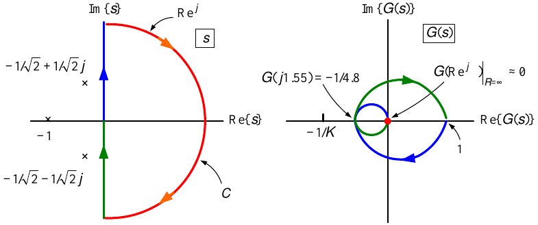
- For what values of \(K>0\) are the zeros of \(\dfrac{1}{K}+G(s)=0\) in the open LHP?
Case (1) Let \(-1/K<-1/4.8\) so \(0<K<4.8.\)
\(P=0\) and we see above that \(N=0\) so
\[Z=N+P=0.\]
Thus \(1/K+G(s)\) has no zeros in the right half-plane for \(0<K<4.8\)
\(\Longrightarrow\) Closed-loop system is stable.
\(G(s)=\dfrac{1}{(s+1)(s^{2}+\sqrt{2}s+1)}\) \(=\dfrac{1}{(s+1)(s-[-1/\sqrt{2}+j/\sqrt{2}])(s-[-1/\sqrt{2}-j/\sqrt{2}])}\)
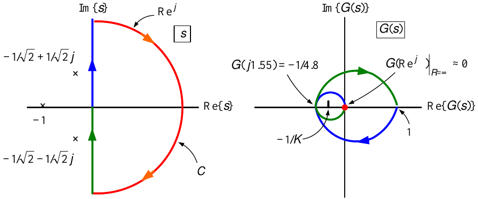
Case (2) Let \(-1/4.8<-1/K\) so \(K>4.8\).
\(P=0\) and from the above plot we see \(N=2.\) Thus
\[Z=N+P=2+0=2.\]
Thus \(1/K+G(s)\) has two zeros in the right half-plane for \(K>4.8.\)
\(\Longrightarrow\) Closed-loop system is unstable.
Check: Apply the Routh-Hurwitz test to \((s+1)(s^{2}+\sqrt{2}s+1)+K=0.\)
Nyquist Stability Test \(G(s)=\dfrac{1}{s(s+1)^{2}}\)
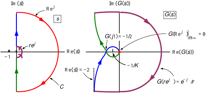
Nyquist Stability Test \(G(s)=\dfrac{1}{s(s+1)^{2}}\)
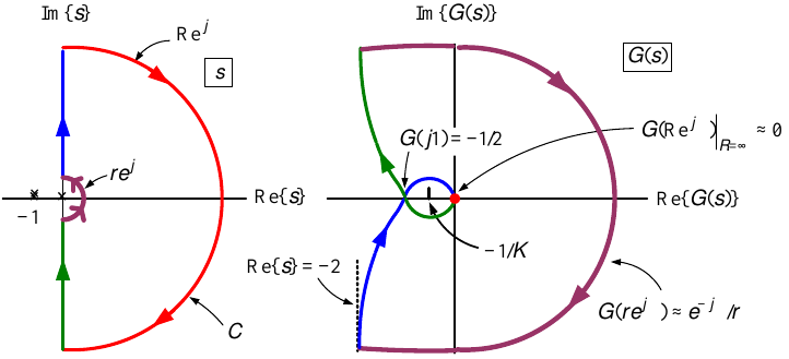
Let \(s=re^{j\theta }\) for \(-\pi /2\leq \theta \leq \pi /2\). Then
\[G(re^{j\theta })=\dfrac{1}{re^{j\theta }(re^{j\theta }+1)^{2}}\approx \dfrac{1}{re^{j\theta }}=\frac{1}{r}e^{-j\theta }\begin{array}{|c|c|} \hline \theta & G(re^{j\theta })\approx \dfrac{1}{r}e^{-j\theta } \\ \hline -\pi /2 & e^{j\pi /2}/r=j/r \\ \hline -\pi /4 & e^{j\pi /4}/r \\ \hline \quad 0 & 1/r \\ \hline +\pi /4 & e^{-j\pi /4}/r \\ \hline +\pi /2 & e^{-j\pi /2}/r=-j/r \\ \hline \end{array}\]
Nyquist Stability Test \(G(s)=\dfrac{1}{s(s+1)^{2}}\)
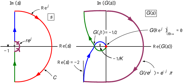
Case (1) Let \(-1/2<-1/K<0\) so \(K>2.\)
\(P=0\) and from the above plot that \(N=2,P=0\) so
\[Z=N+P=2.\]
Thus \(1/K+G(s)\) has two zeros in the right half-plane for \(K>2.\)
\(\Longrightarrow\) Closed-loop system is unstable.
Nyquist Stability Test \(G(s)=\dfrac{1}{s(s+1)^{2}}\)
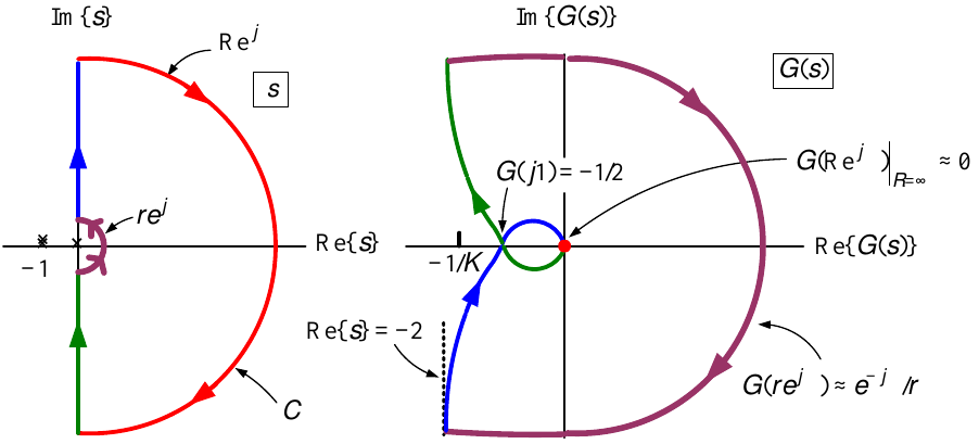
Case (2) Let \(-1/K<-1/2\) so \(0<K<2.\)
\(P=0\) and the above plot shows \(N=0\) so
\[Z=N+P=0.\]
Thus \(1/K+G(s)\) has no zeros in the right half-plane for \(0<K<2.\)
\(\Longrightarrow\) Closed-loop system is stable.
\(G(s)=\dfrac{100(s/10+1)}{s(s-1)(s/100+1)}=-\dfrac{100(s/10+1)}{s(-s+1)(s/100+1)}\)
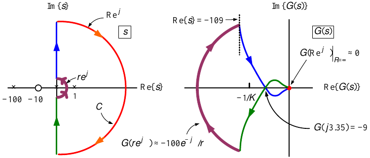
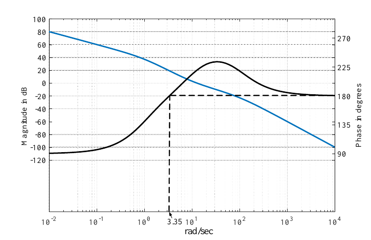
\(G(s)=\dfrac{100(s/10+1)}{s(s-1)(s/100+1)}=-\dfrac{100(s/10+1)}{s(-s+1)(s/100+1)}\)
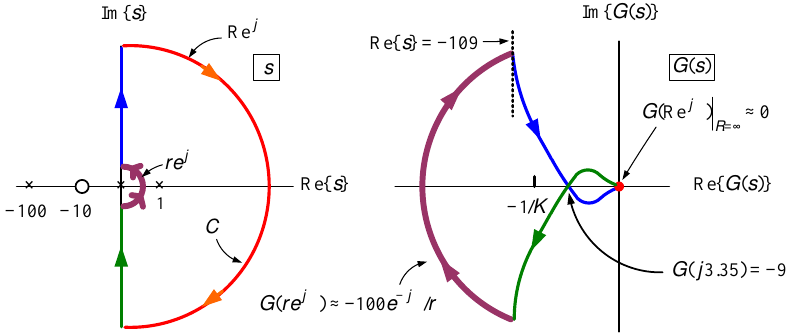
Let \(s=re^{j\theta }\) for \(-\pi /2\leq \theta \leq \pi /2\). Then
\[G(re^{j\theta })=\dfrac{100(re^{j\theta }/10+1)}{re^{j\theta }(re^{j\theta }-1)(re^{j\theta }/100+1)}\approx -\dfrac{100}{re^{j\theta }}=-\frac{100}{r}e^{-j\theta }.\begin{array}{|c|c|} \hline \theta & G(re^{j\theta })\approx -\dfrac{100}{r}e^{-j\theta } \\ \hline -\pi /2 & -100e^{j\pi /2}/r=-j100/r \\ \hline -\pi /4 & -100e^{j\pi /4}/r \\ \hline 0 & -100/r \\ \hline \pi /4 & -100e^{-j\pi /4}/r \\ \hline \pi /2 & -100e^{-j\pi /2}/r=j100/r \\ \hline \end{array}\]
\(G(s)=\dfrac{100(s/10+1)}{s(s-1)(s/100+1)}=-\dfrac{100(s/10+1)}{s(-s+1)(s/100+1)}\)
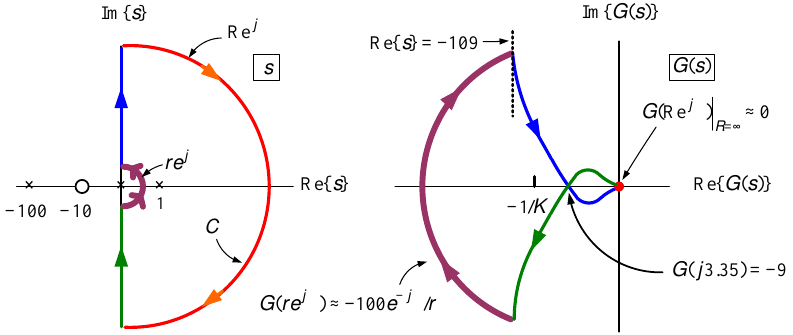
Case (1) \(-1/K<-9\) (\(0<K<1/9\)).
\(P=1\) and from the above plot \(N=1.\) Thus \(Z=N+P=2\).
\(1/K+G(s)\) has two zeros in the right half-plane.
\(\Longrightarrow\) Closed-loop system is unstable for \(0<K<1/9.\)
Case (2) \(-9<-1/K<0\) (\(K>1/9\)).
\(P=1\) and \(N=-1.\) Thus \(Z=N+P=-1+1=0\).
\(1/K+G(s)\) has no zeros in the right half-plane.
\(\Longrightarrow\) Closed-loop system is stable for \(K>1/9.\)
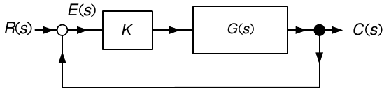
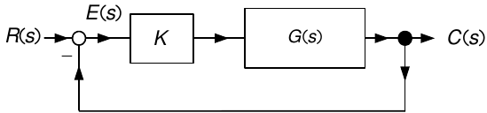
Closed-loop transfer function \(\dfrac{C(s)}{R(s)}=\dfrac{KG(s)}{1+KG(s)}.\)
Closed-loop system is stable iff the zeros of \(1+KG(s)\) are in the open LHP.
The following statements are equivalent:
(1) \(\ G(j\omega ),-\infty <\omega <\infty\) goes around the \(-1/K+j0\) point \(N\) times.
(2) \(\ 1/K+G(j\omega ),-\infty <\omega <\infty\) goes around the origin \(N\) times.
(3) \(\ 1+KG(j\omega ),-\infty <\omega <\infty\) goes around the origin \(N\) times.
(4) \(\ KG(j\omega ),-\infty <\omega <\infty\) goes around the \(-1+j0\) point \(N\) times.
For the concept of gain and phase margins we use statement \(\mathbf{(4)}.\)
\(G(s)=\dfrac{2}{(s+1)(s^{2}+\sqrt{2}s+1)}\) \(=\dfrac{2}{(s+1)(s-[-1/\sqrt{2}+j/\sqrt{2}])(s-[-1/\sqrt{2}-j/\sqrt{2}])}\)
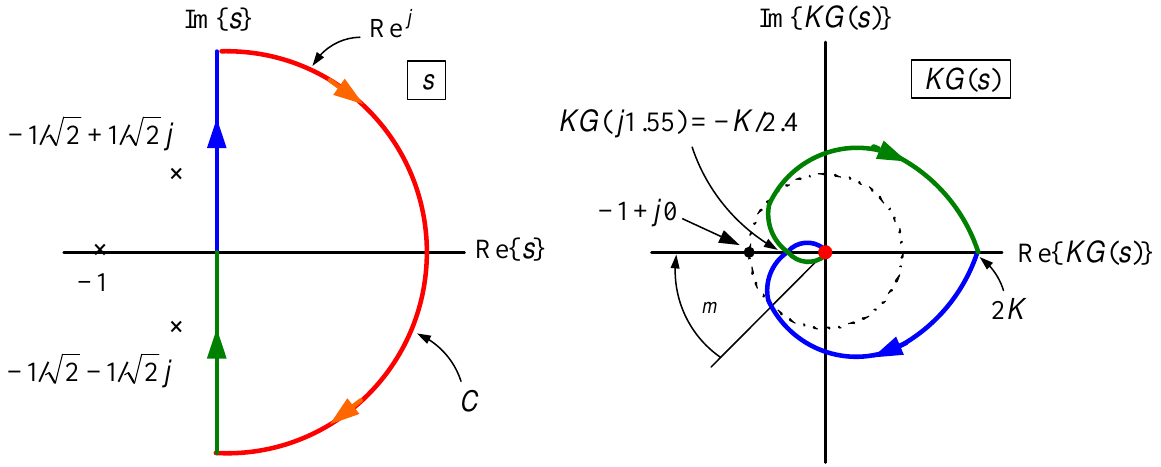
- \(\angle G(j1.55)=180^{\circ },\) \(\ G(j1.55)=-1/2.4\)
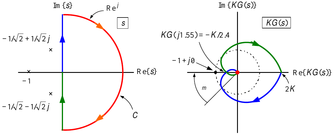
\(P=0\) and the Nyquist plot does not encircle the \(-1+j0\) point for \(0<K<2.4\).
\(\Longrightarrow 1+KG(s)=0\) does not have any zeros in the right half-plane for \(0<K<2.4\).
\(G(s)=\dfrac{2}{(s+1)(s^{2}+\sqrt{2}s+1)}\) \(=\dfrac{2}{(s+1)(s-[-1/\sqrt{2}+j/\sqrt{2}])(s-[-1/\sqrt{2}-j/\sqrt{2}])}\)
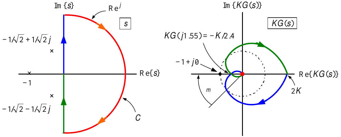
We just showed the closed-loop system is stable for \(0<K<2.4.\)
The gain \(K\) can be increased to 2.4 before the system becomes unstable.
We say the gain margin is 2.4 or, in decibels, it is \(20\log _{10}2.4=7.6\) dB.
\(G(s)=\dfrac{2}{(s+1)(s^{2}+\sqrt{2}s+1)},\) \(G(j1)=\dfrac{2}{\sqrt{2}e^{j\pi /4}(\sqrt{2}j)}=1e^{-j3\pi /4}\)
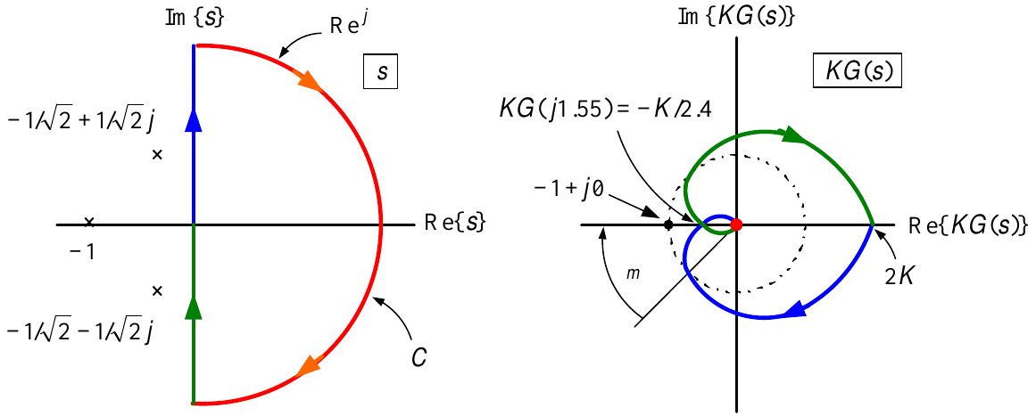
Note the (dashed) circle of radius 1 centered at the origin.
\(\omega _{g}\) is the value of \(\omega\) for which \(|G(j\omega _{g})|=1.\) Here \(\omega _{g}=1\) and \(G(j\omega _{g})=1e^{-j3\pi /4}.\)
The angle \(\phi _{m}\) between \(G(j\omega _{g})\) and the neg real axis is the phase margin, i.e.,
\[\phi _{m}=\angle G(j\omega _{g})+180^{\circ }=-135^{\circ }+180^{\circ }=45^{\circ }.\]
The phase margin is how much the Nyquist plot can be rotated before it encloses the \(-1+j0\) point.
\(G(s)=\dfrac{2}{(s+1)(s^{2}+\sqrt{2}s+1)}\) \(=\dfrac{2}{(s+1)(s-[-1/\sqrt{2}+j/\sqrt{2}])(s-[-1/\sqrt{2}-j/\sqrt{2}])}\)
Definition Gain Crossover Frequency \(\omega _{g}\)
A gain crossover frequency is a frequency \(\omega _{g}\) at which
\[|G(j\omega _{g})|=1\;\iff \;20\log |G(j\omega _{g})|=0.\]
Definition Phase Crossover Frequency \(\omega _{\phi }\)
A phase crossover frequency is a frequency \(\omega _{\phi }\) at which
\[\angle G(j\omega _{\phi })=-180^{\circ }.\]
\(G(s)=\dfrac{2}{(s+1)(s^{2}+\sqrt{2}s+1)}\)
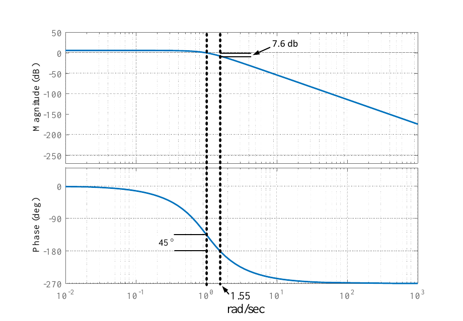
The phase crossover frequency is \(\omega _{\phi }=1.55.\)
\(20\log _{10}|G(j1.55)|=20\log _{10}|-1/2.4|=-7.6\) dB.
\(\Longrightarrow\) Gain margin is \(7.6\) dB.
The gain crossover frequency is \(\omega _{g}=1\) and \(G(j\omega _{g})=G(j1)=1e^{-j3\pi /4}=1e^{-j135^{\circ }}.\)
\(\Longrightarrow\) Phase margin is \(45^{\circ }.\)
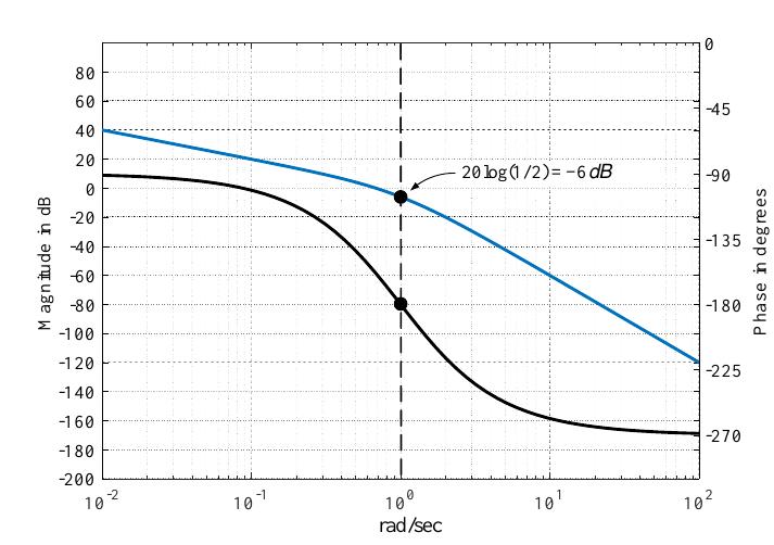
\(G(s)=\dfrac{1}{s(s+1)^{2}}\)
\(\omega _{g}=1\) and \(G(j\omega _{g})=G(j1)=-1/2.\)
\(\omega _{\phi }=0.68\) and \(G(j\omega _{\phi })=G(j0.68)=1e^{-j159^{\circ }}\)
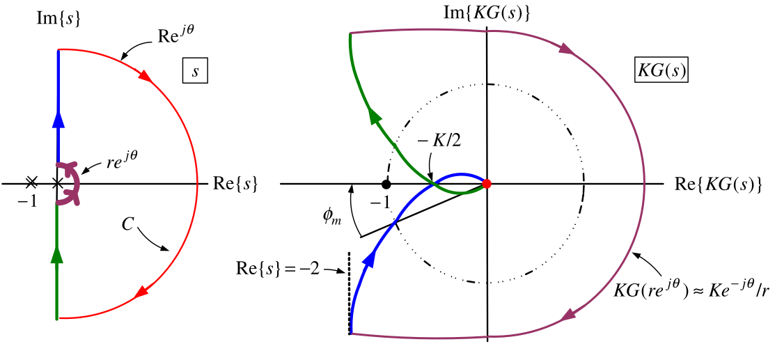
\(P=0\)
For \(0<K<2,\) we have \(N=0\) and thus \(Z=N+P=0.\) Stable!
For \(K>2\) we have \(N=2\) and thus \(Z=N+P=2.\) Unstable!
The gain margin is \(20\log _{10}2=6.02\) dB\(.\)
The phase margin is \(\phi _{m}=\angle G(j\omega _{g})+180=-159^{\circ }+180^{\circ }=21^{\circ }.\)
\(G(s)=\dfrac{1}{s(s+1)^{2}}\)
.
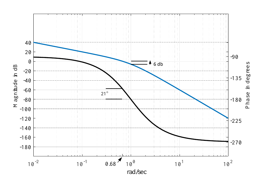
Important information at the crossover frequencies:
\[\begin{array}{|l|l|l|} \hline \omega _{g}=0.68 & 20\log _{10}|G(j\omega _{g})|=0 dB & \angle G(j\omega _{g})=-159^{\circ } \\ \hline \omega _{\phi }=1 & 20\log _{10}|G(j\omega _{\phi })|=20\log _{10}(1/2)=-6 dB & \angle G(j\omega _{\phi })=-180^{\circ } \\ \hline \end{array}\]
\(G(s)=\dfrac{100(s/10+1)}{s(s-1)(s/100+1)},\) \(\ G(j3.35)=-9,\) \(\ G(j12.6)=1e^{-j140^{\circ }}\)
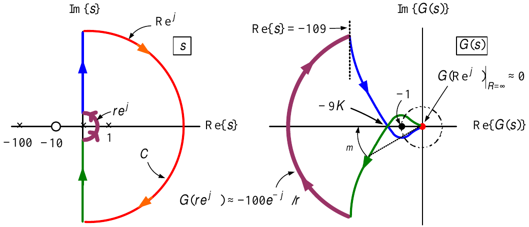
\[\begin{array}{|l|l|l|} \hline \omega _{g}=12.6 & 20\log _{10}|G(j\omega _{g})|=0 dB & \angle G(j\omega _{g})=-140^{\circ } \\ \hline \omega _{\phi }=3.35 & 20\log _{10}|G(j\omega _{\phi })|=20\log _{10}(|-9|)=19.1 dB & \angle G(j\omega _{\phi })=-180^{\circ }. \\ \hline \end{array}\]
\(P=1\)
For \(K>1/9\) we have \(N=-1\) and thus \(Z=N+P=-1+1=0.\) Stable!
For \(K<1/9\) we have \(N=+1\) and thus \(Z=N+P=\quad \!1+1=2.\) Unstable!
\(G(s)=\dfrac{100(s/10+1)}{s(s-1)(s/100+1)}\)
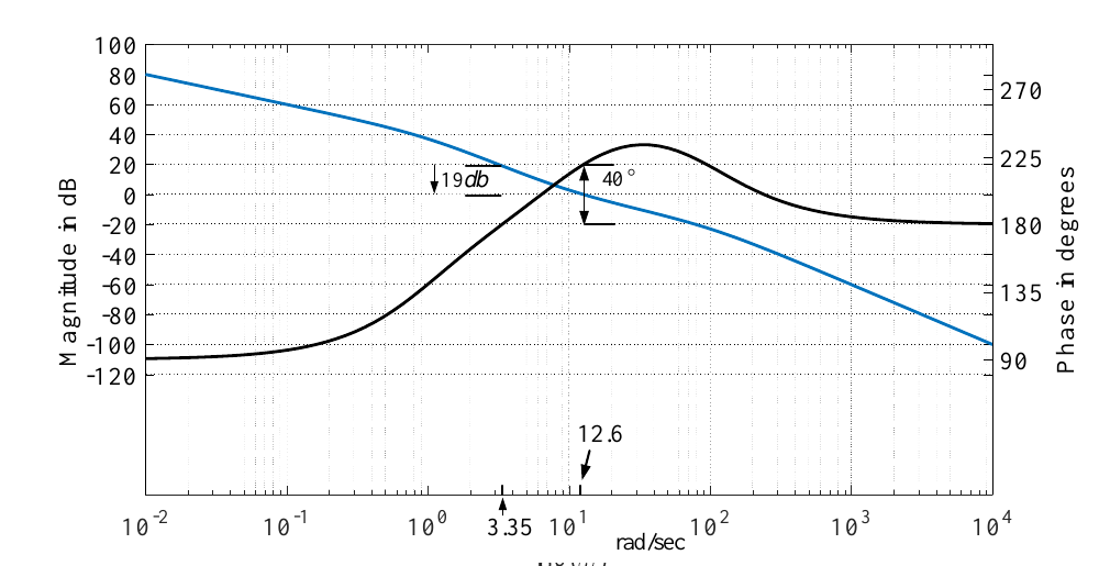
Here the gain margin is the amount \(K\) can reduced before becoming unstable.
The gain margin is \(20\log _{10}(1/9)=-19.1\) dB
At the gain crossover frequency \(\omega _{g}=12.6\) and \(\angle G(j\omega _{g})=\angle G(j12.6)=-140^{\circ }.\)
Nyquist plot can be rotated by \(40^{\circ }\) before becoming unstable.
The phase margin is \(40^{\circ }.\)
\(y(t)\)
may be written as
\[y(t)=\frac{1}{2\pi }\int_{-\infty }^{+\infty }Y(j\omega )e^{j\omega t}d\omega =\frac{1}{2\pi }\int_{-\infty }^{+\infty }T(j\omega )R(j\omega )e^{j\omega t}d\omega .\]
\(R(j\omega )d\omega\) is the frequency content of \(r(t)\) between \(\omega\) and \(\omega +d\omega .\)
The frequency content of \(y(t)\) in this same interval is \(T(j\omega )R(j\omega )d\omega .\)
\(y(t)\) is the sum (integral) of the pure sinusoids \(T(j\omega )R(j\omega )e^{j\omega t}d\omega .\)
The goal is to have \(y(t)\) track \(r(t)\).
Need to find \(G_{c}(j\omega )\) so that the closed-loop transfer function
\[T(j\omega )=\dfrac{G_{c}(j\omega )G(j\omega )}{1+G_{c}(j\omega )G(j\omega )}\]
satisfies
\[T(j\omega )\approx \left\{ \begin{array}{cl} 1, & |\omega |\leq \omega _{B} \\ 0, & |\omega |>\omega _{B}.\end{array}\right.\]
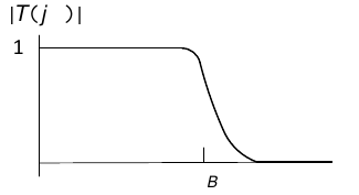
\(\omega _{B}\) is the bandwidth of the closed-loop system.
\[T(j\omega )=\dfrac{G_{c}(j\omega )G(j\omega )}{1+G_{c}(j\omega )G(j\omega )}\;\text{with}\;T(j\omega )\approx \left\{ \begin{array}{cl} 1, & |\omega |\leq \omega _{B} \\ 0, & |\omega |>\omega _{B}.\end{array}\right.\]
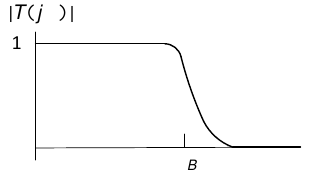
Tracking: Suppose \(R(j\omega )\approx 0\) for \(|\omega |>\omega _{B}\).
\[\begin{aligned} \!\!\!\!y(t)=\frac{1}{2\pi }\!\!\int\limits_{-\infty }^{+\infty }\!\!\!T(j\omega )R(j\omega )e^{j\omega t}d\omega \!\!\!\!\! &\!\!\approx \!\!\!\!\!&\!\!\frac{1}{2\pi }\!\!\int\limits_{-\omega _{B}}^{+\omega _{B}}\!\!\!T(j\omega )R(j\omega )e^{j\omega t}d\omega \;\text{as}\;R(j\omega )\approx 0\;\text{for}\;|\omega |\!>\omega _{B} \\ &\approx &\frac{1}{2\pi }\int\limits_{-\omega _{B}}^{+\omega _{B}}R(j\omega )e^{j\omega t}d\omega \;\text{as}\;T(j\omega )\approx 1\;\text{for}\;|\omega |\leq \omega _{B} \\ &\approx &\frac{1}{2\pi }\int\limits_{-\infty }^{+\infty }R(j\omega )e^{j\omega t}d\omega \;\text{as}\;R(j\omega )\approx 0\;\text{for}\;|\omega |>\omega _{B} \\ &\approx &r(t). \end{aligned}\]
- Design the controller so \(T(j\omega )\approx 1\) for \(|\omega |\leq \omega _{B}\) and \(T(j\omega )\approx 0\) for \(|\omega |>\omega _{B}.\)
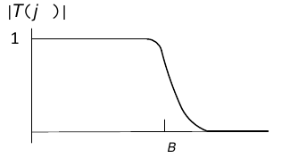
If \(R(j\omega )\approx 0\) for \(|\omega |>\omega _{B}\), then should have good tracking.
With \(T(s)\) stable and \(r(t)=R_{0}\cos (\omega t)\),
\[y(t)\rightarrow y_{ss}(t)=|T(j\omega )|R_{0}\cos (\omega t+\angle T(j\omega ))\approx R_{0}\cos (\omega t)\;\text{for}\;|\omega |\leq \omega _{B}.\]
A typical reference is a step input. Unit step does not have a Fourier transform.
\[\int_{-\infty }^{\infty }u_{s}(t)e^{-j\omega t}dt=\int_{0}^{\infty }u_{s}(t)e^{-j\omega t}dt=\left. \frac{e^{-j\omega t}}{-j\omega }\right\vert _{0}^{\infty }=\underset{\text{does not converge}}{\underbrace{\lim_{t\rightarrow \infty }\frac{e^{-j\omega t}}{-j\omega }}}+\frac{1}{j\omega }\text{.}\]
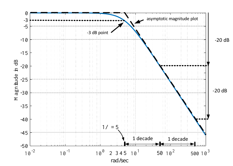
Bode Diagam of \(T(j\omega )=\dfrac{1}{\tau j\omega +1}=\dfrac{1/\tau }{j\omega +1/\tau }.\)
\(\tau =0.2\)
\(\omega _{b}=1/\tau =5\) as \(|T(j5)|=1/\sqrt{2}\) or \(20\log _{10}(|T(j5)|)=\) \(-3\) dB.
\(p=-1/\tau =-5.\) The further in the LFP the pole resides, the larger the bandwidth.
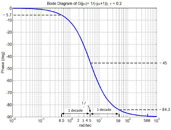
Bode Diagam of \(\angle T(j\omega )=\angle \dfrac{1}{\tau j\omega +1}=\angle \dfrac{1/\tau }{j\omega +1/\tau }.\)
\(\tau =0.2\)
\(\omega _{b}=1/\tau =5\) as \(|T(j5)|=1/\sqrt{2}\) or \(20\log _{10}(|T(j5)|)=\) \(-3\) dB.
The angle plot shows the frequency must be below \(0.1\omega _{B}\) for \(\angle T(j\omega )\approx 0.\)
That is, \(T(j\omega )\approx 1\) is only reasonable for \(|\omega |<0.1\omega _{B}.\)
Bode diagram of \(T(s)=\dfrac{\omega _{n}^{2}}{s^{2}+2\zeta \omega _{n}s+\omega _{n}^{2}}\) with \(\omega _{n}=1,\zeta =0.1\).
The closed-loop poles are at \(p_{i}=-\zeta \omega _{n}\pm j\omega _{n}\sqrt{1-\zeta ^{2}}.\)
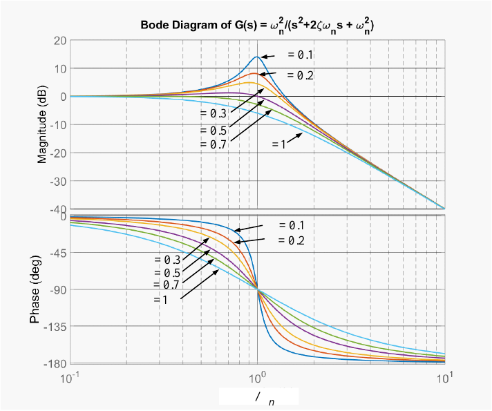
Normally the CL poles are placed so that \(\zeta \geq 0.6\).
At \(\omega _{n}\) we have \(|G(j\omega _{n})|=1/(2\zeta ).\)
At \(\omega _{n}\) with \(\zeta\) to \(1,\) the magnitude plot is down by \(1/2\) (\(-6\) dB)
At \(\omega _{n}\) with \(\zeta =0.6,\) the magnitude plot is down by \(1/1.2\) (\(-1.6\) dB).
For convenience just take the bandwidth to be \(\omega _{B}=\omega _{n}.\)
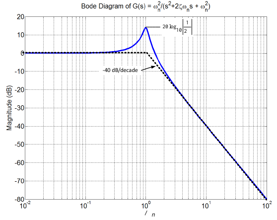
Bode diagram of \(T(s)=\dfrac{\omega _{n}^{2}}{s^{2}+2\zeta \omega _{n}s+\omega _{n}^{2}}\) with \(\omega _{n}=1\).
For convenience just take the bandwidth to be \(\omega _{B}=\omega _{n}.\)
The phase plot shows \(\omega \leq 0.1\omega _{B}=0.1\omega _{n}\) for \(\angle T(j\omega )\approx 0.\)
That is, \(T(j\omega )\approx 1\) is only reasonable for \(|\omega |<0.1\omega _{B}.\)
The further the poles are in the left half-plane and the larger the bandwidth.
Choose \(G_{c}(s)\) so \(T(s)=\dfrac{G_{c}(s)G(s)}{1+G_{c}(s)G(s)}\) has the desired shape.
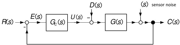
\[C(s)=\underset{T(s)}{\underbrace{\frac{G_{c}(s)G(s)}{1+G_{c}(s)G(s)}}}R(s)-\frac{G(s)}{1+G_{c}(s)G(s)}D(s)+\underset{S(s)}{\underbrace{\frac{1}{1+G_{c}(s)G(s)}}}\eta (s).\]
\(G(s)\) strictly proper and \(G_{c}(s)\) (at least) proper.
\[|G_{c}(j\omega )G(j\omega )|\rightarrow 0\;\text{as}\;|\omega |\rightarrow \infty .\]
Need \(|G_{c}(j\omega )G(j\omega )|>>1\) for \(|\omega |\leq \omega _{B}\) so that
\[T(j\omega )=\frac{G_{c}(j\omega )G(j\omega )}{1+G_{c}(j\omega )G(j\omega )}\approx \frac{G_{c}(j\omega )G(j\omega )}{G_{c}(j\omega )G(j\omega )}=1\;\text{for}\;|\omega |\leq \omega _{B}.\]
If the controller has an integrator then \(|G_{c}(j\omega )G(j\omega )|\rightarrow \infty\) as \(|\omega |\rightarrow 0.\)
Need \(|G_{c}(j\omega )G(j\omega )|\rightarrow 0\) fast for \(|\omega |>\omega _{B}\) so that
\[T(j\omega )=\frac{G_{c}(j\omega )G(j\omega )}{1+G_{c}(j\omega )G(j\omega )}\approx 0\;\text{for}\;|\omega |>\omega _{B}.\]
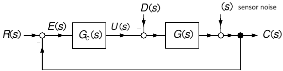
\[C(s)=\underset{T(s)}{\underbrace{\frac{G_{c}(s)G(s)}{1+G_{c}(s)G(s)}}}R(s)-\frac{G(s)}{1+G_{c}(s)G(s)}D(s)+\underset{S(s)}{\underbrace{\frac{1}{1+G_{c}(s)G(s)}}}\eta (s).\]
Want the bandwidth \(\omega _{B}\) large enough so that \(R(j\omega )\approx 0\) for \(|\omega |>\omega _{B}.\)
Then
\[C_{R}(j\omega )\triangleq \frac{G_{c}(j\omega )G(j\omega )}{1+G_{c}(j\omega )G(j\omega )}R(j\omega )\approx R(j\omega ).\]
Disturbance rejection follows if \(|G_{c}(j\omega )|>>1\) for \(|\omega |<\omega _{B}\) as
\[C_{D}(j\omega )\triangleq -\frac{G(j\omega )}{1+G_{c}(j\omega )G(j\omega )}D(s)\approx -\frac{1}{G_{c}(j\omega )}D(j\omega )\approx 0\;\text{for}\;|\omega |<\omega _{B}.\]
As \(|G_{c}(j\omega )G(j\omega )|\rightarrow 0\) as \(|\omega |\rightarrow \infty ,\) we also have \(|C_{D}(j\omega )|\rightarrow 0\) as \(|\omega |\rightarrow \infty .\)
Tracking and dist rej achievable using a strictly proper stabilizing controller \(G_{c}(j\omega )\)
with \(|G_{c}(j\omega )|>>1\) for \(|\omega |<\omega _{B}\) and \(|G_{c}(j\omega )|\rightarrow 0\) rapidly for \(|\omega |>\omega _{B}\)
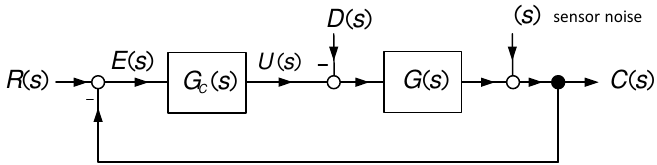
\[C(s)=\underset{T(s)}{\underbrace{\frac{G_{c}(s)G(s)}{1+G_{c}(s)G(s)}}}R(s)-\frac{G(s)}{1+G_{c}(s)G(s)}D(s)+\underset{S(s)}{\underbrace{\frac{1}{1+G_{c}(s)G(s)}}}\eta (s).\]
Effect of the measurement noise on output.
\[C_{\eta }(j\omega )\triangleq \frac{1}{1+G_{c}(j\omega )G(j\omega )}\eta (j\omega )\approx \left\{ \begin{array}{cl} 0 & |\omega |\leq \omega _{B} \\ \eta (j\omega ) & |\omega |>\omega _{B}.\end{array}\right.\]
Low-frequency noise is attenuated by feedback.
High frequency noise is essentially unchanged.
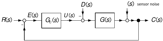
Low-frequency sensor noise is a problem for the actuator!.
The output of the controller \(U_{\eta }(s)\) (actuator command) due to \(\eta (s)\) is
\[U_{\eta }(s)\triangleq -\frac{G_{c}(j\omega )}{1+G_{c}(j\omega )G(j\omega )}\eta (j\omega )\approx \left\{ \begin{array}{ll} -\dfrac{1}{G(j\omega )}\eta (j\omega ) & |\omega |\leq \omega _{B} \\ -G_{c}(j\omega )\eta (j\omega )\rightarrow 0 & |\omega |>\omega _{B}.\end{array}\right.\]
As \(G(s)\) is strictly proper, \(1/G(s)\) is non proper resulting in the low-frequency noise being differentiated.
E.g., \(G(s)=\dfrac{b}{s(s+a)},\) \(-\eta (s)/G(s)=-\dfrac{1}{b}(s^{2}+as)\eta (s)\) so \(\eta (s)\) is differentiated twice.
Important to have sensors with essentially no noise for \(|\omega |\leq \omega _{B}.\)
The closed-loop bandwidth must be chosen so that it
does not contain any significant frequency content of \(\eta (j\omega ).\)
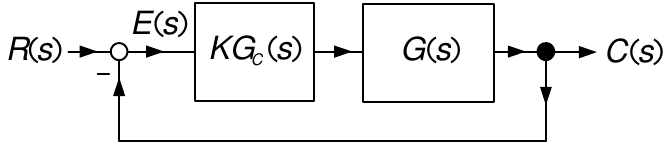
Let \(G_{c}(s)=1\) so it is simply a proportional feedback control problem.
Let
\[G(s)=\frac{1}{(s+1)(s+2)(s+4)},\;R(s)=\frac{1}{s}.\]
If the closed-loop system is stable then
\[\begin{aligned} e(\infty )=\lim_{s\rightarrow 0}s\frac{1}{1+K\dfrac{1}{(s+1)(s+2)(s+4)}}\frac{1}{s} &=&\lim_{s\rightarrow 0}\frac{1}{1+K\dfrac{1}{(s+1)(s+2)(s+4)}} \\ &=&\frac{1}{1+K/8}. \end{aligned}\]
The larger the gain the smaller the steady-state error.
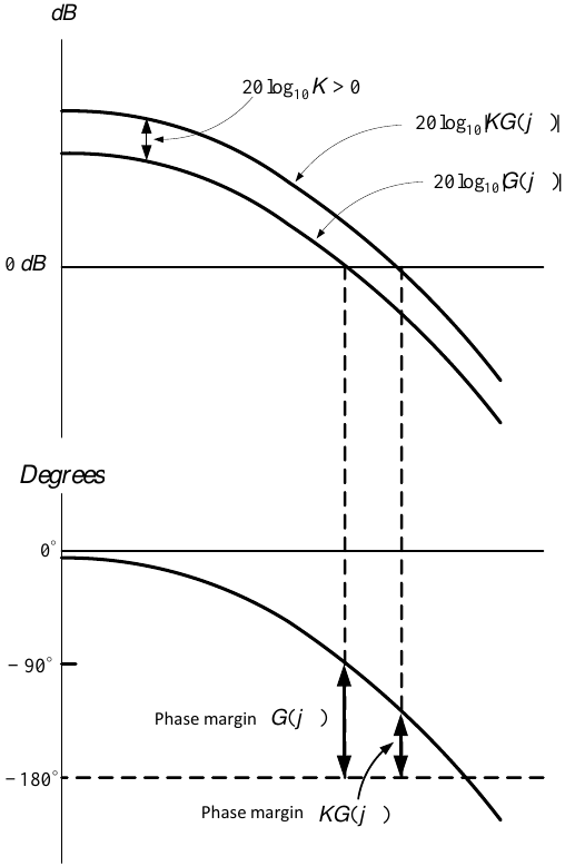
However, increasing the open-loop gain \(K\) usually decreases the phase margin.
\(G(s)=\dfrac{1}{(s+1)(s+2)(s+4)}\)
- Increasing the gain too much makes the closed-loop system unstable.
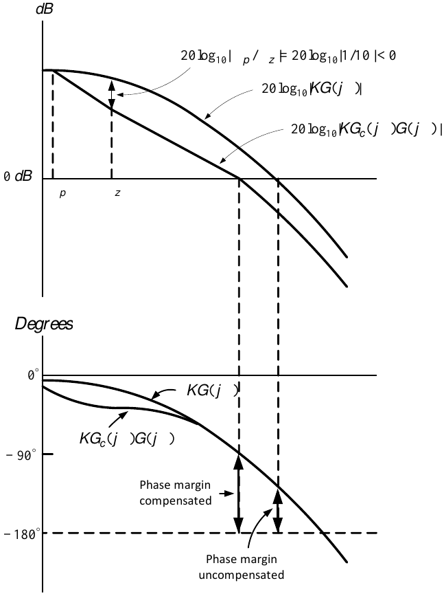
\(G_{c}(s)=\dfrac{0.01}{0.1}\dfrac{s+0.1}{s+0.01}=\dfrac{s/0.1+1}{s/0.01+1}\)
- \(KG_{c}(0)=K\) and \(KG_{c}(j\omega )\rightarrow \dfrac{K}{10}\) as \(\omega \rightarrow \infty .\)
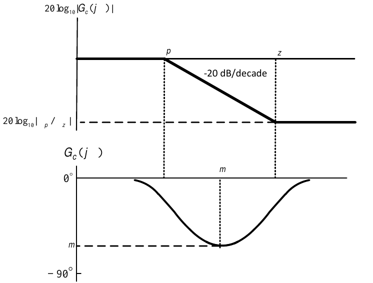
- \(\omega _{p}=0.01,\) \(\omega _{z}=0.1\) and \(\ \omega _{p}<\omega _{z}<<\omega _{g}.\)
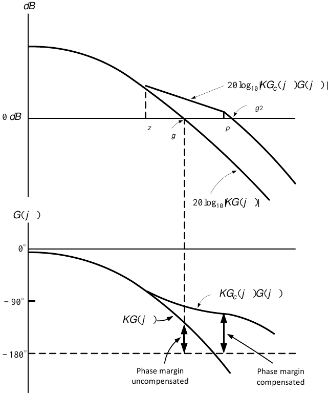
\[\begin{aligned} G_{c}(s) &=&\frac{s/\omega _{z}+1}{s/\omega _{p}+1}=\frac{\omega _{p}}{\omega _{z}}\frac{s+\omega _{z}}{s+\omega _{p}}\;\text{where}\;\omega _{z}<\omega _{p} \\ KG_{c}(0) &=&K \\ KG_{c}(j\omega ) &\rightarrow &\frac{\omega _{p}}{\omega _{z}}K>K\;\text{as}\;\omega \rightarrow \infty . \end{aligned}\]
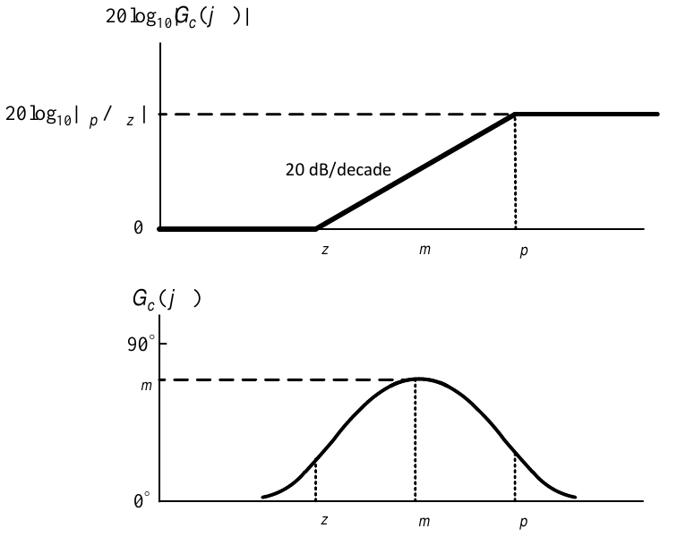
- Key Requirement of Lead Compensators: \(\omega _{z}<\omega _{g}<\omega _{p}\)
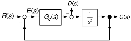
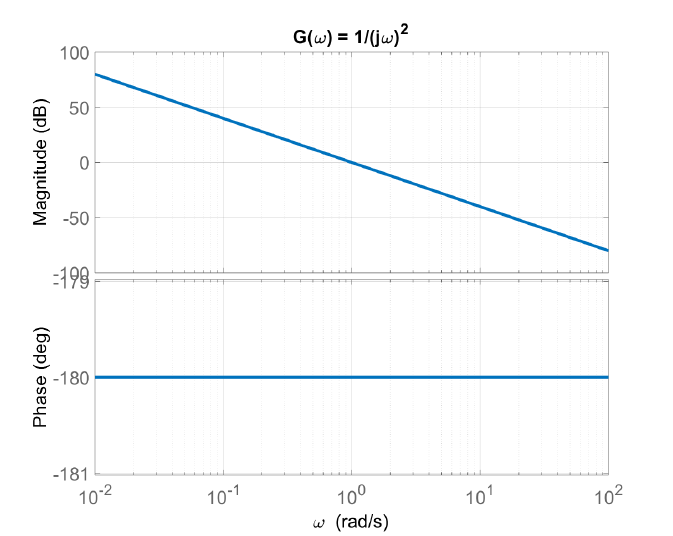
- The gain crossover frequency is \(\omega _{cg}=1\) rad/sec
- Bode diagram of \(G_{c}(s)G(s)=10\dfrac{s+0.1}{s+10}\dfrac{1}{s^{2}}\).
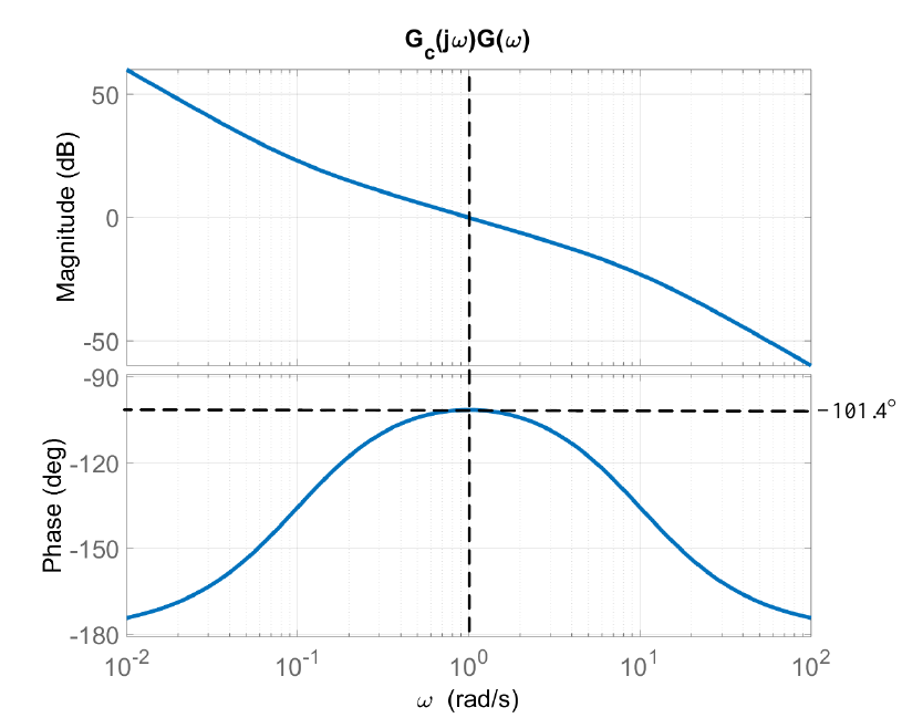
- At \(\omega =\omega _{cg}=1,G_{c}(j\omega )G(j\omega )=1e^{-j101.4^{\circ }}\) so the PM is \(180^{\circ }-101.4^{\circ }=78.6^{\circ }.\)
The Nyquist contour for \(G_{c}(s)G(s)=10\dfrac{s+0.1}{s+10}\dfrac{1}{s^{2}}\).
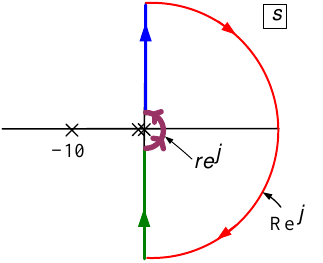
Nyquist contour shows \(P=0.\)
For \(s=re^{j\theta }\) with \(r\) small \(\ G_{c}(re^{j\theta })G(re^{j\theta })=10\dfrac{re^{j\theta }+0.1}{re^{j\theta }+10}\dfrac{1}{r^{2}e^{j2\theta }}\approx \dfrac{0.1}{r^{2}}e^{-j2\theta }.\)
\[\begin{array}{|c|l|} \hline \theta & G(re^{j\theta })G_{c}(re^{j\theta })\approx 0.1e^{-j2\theta }/r^{2} \\ \hline -\pi /2 & 0.1e^{j180^{\circ }}/r^{2} \\ \hline -\pi /4 & 0.1e^{j90^{\circ }}/r^{2} \\ \hline 0 & 0.1/r^{2} \\ \hline +\pi /4 & 0.1e^{-j90^{\circ }}/r^{2} \\ \hline +\pi /2 & 0.1e^{-j180^{\circ }}/r^{2} \\ \hline \end{array}\]
.
Polar plot for \(G_{c}(s)G(s)=10\dfrac{s+0.1}{s+10}\dfrac{1}{s^{2}}.\)
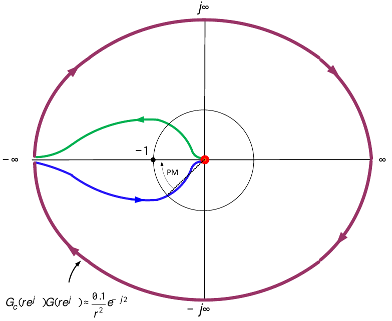
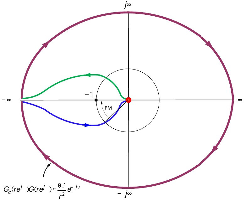
\(P=0\) and \(N=0\) \(\ \Longrightarrow\) \(\ \ Z=N+P=0.\)
By inspection the gain margin is infinite.
The phase margin is \(78.6^{\circ }\) (via Matlab)
\(\ G_{c}(s)G(s)=\dfrac{s+0.1}{s+0.01}10\dfrac{s+0.1}{s+10}\dfrac{1}{s^{2}}\)
Phase margin is \(73.5^{\circ }.\)
\(\left\vert \dfrac{j\omega +0.1}{j\omega +0.01}\right\vert _{\omega =\omega _{cg}=1}=1.005\) and \(\left. \angle \dfrac{j\omega +0.1}{j\omega +0.01}\right\vert _{\omega =\omega _{cg}=1}=-5.1^{\circ }\).
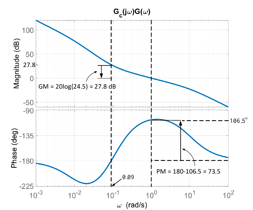
\(\ G_{c}(s)G(s)=\dfrac{s+0.1}{s+0.01}10\dfrac{s+0.1}{s+10}\dfrac{1}{s^{2}}\)
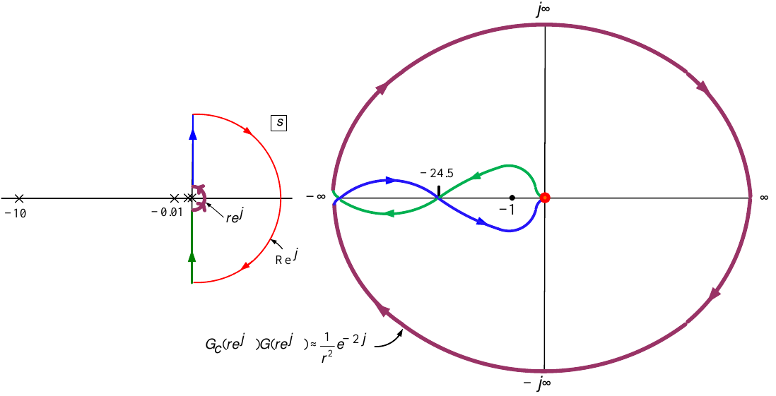
\(G(re^{j\theta })G_{c}(re^{j\theta })=\dfrac{re^{j\theta }+0.1}{re^{j\theta }+0.01}10\dfrac{re^{j\theta }+0.1}{re^{j\theta }+10}\dfrac{1}{r^{2}e^{j2\theta }}\approx \dfrac{1}{r^{2}}e^{-j2\theta }\).
\(P=0,Z=0\rightarrow N=Z-P=0.\ \)
Phase margin is \(73.5^{\circ }.\)
Gain margin \(1/24.5=0.0408\) or \(20\log (0.0408)=-27.8\) dB.
The lag compensator has decreased the phase and gain margins.
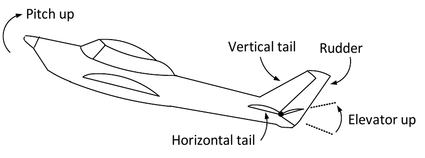
\[G(s)=\frac{\theta (s)}{\delta (s)}=\dfrac{1.51s+0.1774}{s^{3}+0.739s^{2}+0.921s}=\dfrac{1.51s+0.1774}{s(s^{2}+0.739s+0.9597)}.\]
Design specifications
(1) Overshoot less than \(10\%\)
(2) Rise time less than \(2\) seconds
(3) Settling time less than \(10\) seconds
(4) Steady-state error less than \(2\%\) for a step input.
(5) Maximum elevator deflection is \(25^{\circ }\) (\(0.436\) radians), i.e., \(-25^{\circ }\leq \delta \leq 25^{\circ }.\)
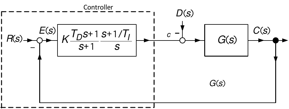
Consider a cascade PID controller
\[G_{c}(s)=K\frac{T_{D}s+1}{\tau s+1}\frac{s+1/T_{I}}{s}.\]
Then
\[20\log (|G_{c}(j\omega )|)=20\log (K)+20\log \left( \left\vert \frac{T_{D}j\omega +1}{\tau j\omega +1}\right\vert \right) +20\log \left( \left\vert \frac{j\omega +1/T_{I}}{j\omega }\right\vert \right) .\]
\(G(s)=\dfrac{1.51s+0.1774}{s^{3}+0.739s^{2}+0.921s}=\dfrac{1.51(s+0.1175)}{s(s^{2}+2\zeta \omega _{n}s+\omega _{n}^{2})},\) \(\zeta =0.377\) & \(\omega _{n}=0.9796\)
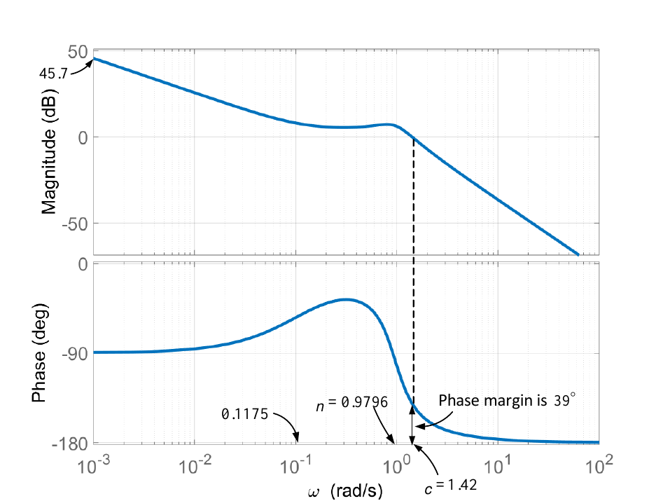
If \(G_{c}(s)=K=1\) then the gain crossover frequency is \(\omega _{cg}=1.42.\)
\(G(j1.42)=1e^{-141^{\circ }}\) giving a phase margin of \(39^{\circ }.\)
\(G(s)=\dfrac{1.51s+0.1774}{s^{3}+0.739s^{2}+0.921s}\rightarrow \dfrac{1.51}{0.921}+\dfrac{0.1774}{0.921}\dfrac{1}{s}\)
as \(|s|\rightarrow 0.\)
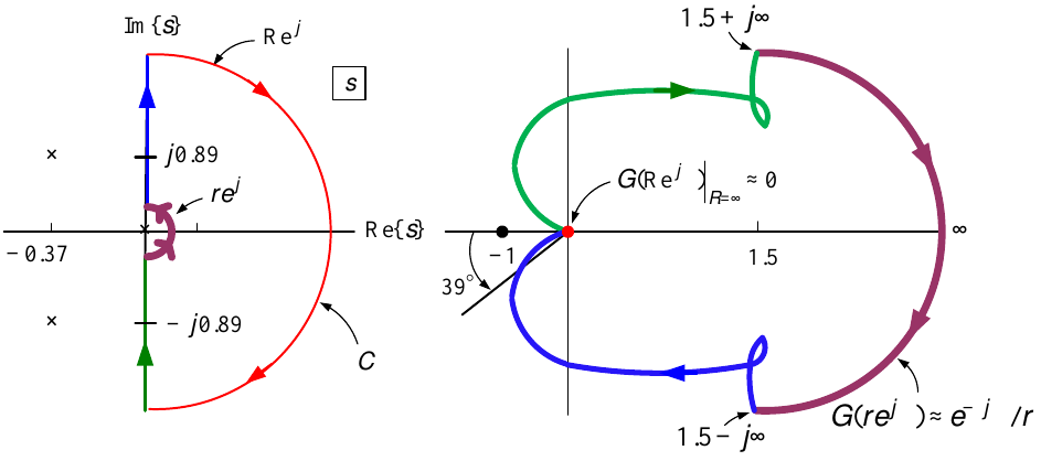
Consider \(G_{c}(s)=\dfrac{s+1/T_{I}}{s}.\)
Require \(1/T_{I}<<\omega _{c}=1.42\) so that at the crossover frequency \(\omega _{c}=1.42\).
\[\dfrac{s+1/T_{I}}{s}|_{s=j\omega _{c}}\approx 1.\]
Set \(T_{I}=10\) so \(1/T_{I}=0.1<<\omega _{c}=1.42\) so \(\ G_{c}(s)=\dfrac{s+0.1}{s}.\)
\(G_{c}(s)G(s)=\dfrac{s+0.1}{s}\dfrac{1.51s+0.1774}{s^{3}+0.739s^{2}+0.921s}\)
The crossover frequency is still at \(1.42.\)
The phase margin is reduced to \(35^{\circ }.\)
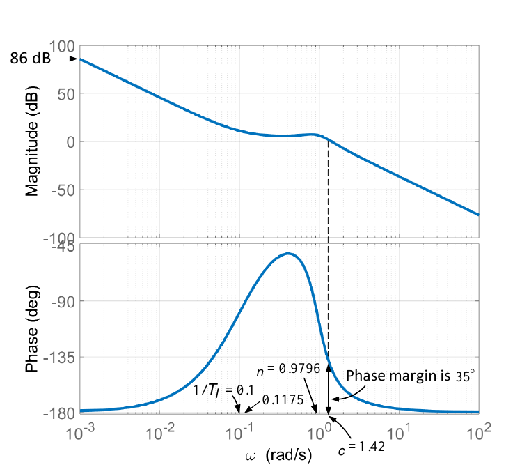
\(G_{c}(s)G(s)=\dfrac{s+0.1}{s}\dfrac{1.51s+0.1774}{s^{3}+0.739s^{2}+0.921s}\)
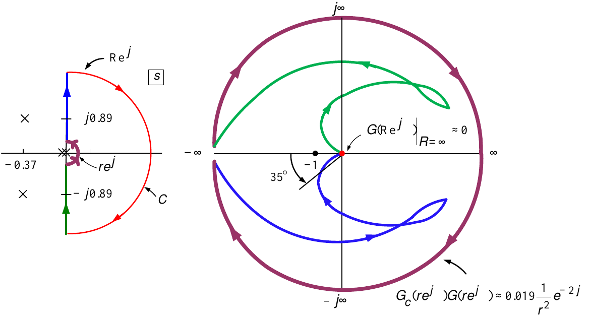
\(G_{c}(re^{j\theta })G(re^{j\theta })\overset{r\rightarrow 0}{\rightarrow }0.1\dfrac{1}{re^{j\theta }}\dfrac{0.1774}{0.921}\dfrac{1}{re^{j\theta }}=0.019\dfrac{1}{r^{2}}e^{-j2\theta }\).
\(T_{D}s+1\)
\(\angle (T_{D}j\omega +1)|_{\omega =1/T_{D}}=45^{\circ }\) and \(20\log |T_{D}j\omega +1)|_{\omega =1/T_{D}}=3\) dB \(\approx 0\).
Set \(1/T_{D}\) of \(T_{D}s+1\) close to \(\omega _{c}=1.42\) to increase the phase margin.
Set \(T_{D}=1/1.42=0.704\) so \(G_{c}(s)=(0.704s+1)\dfrac{s+0.1}{s}.\)
Bode diagram for \(G_{c}(s)G(s)=(0.704s+1)\dfrac{s+0.1}{s}\dfrac{1.51s+0.1774}{s^{3}+0.739s^{2}+0.921s}.\)
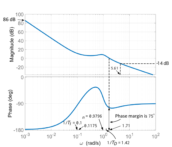
\(G_{c}(s)G(s)=(0.704s+1)\dfrac{s+0.1}{s}\dfrac{1.51s+0.1774}{s^{3}+0.739s^{2}+0.921s}\)
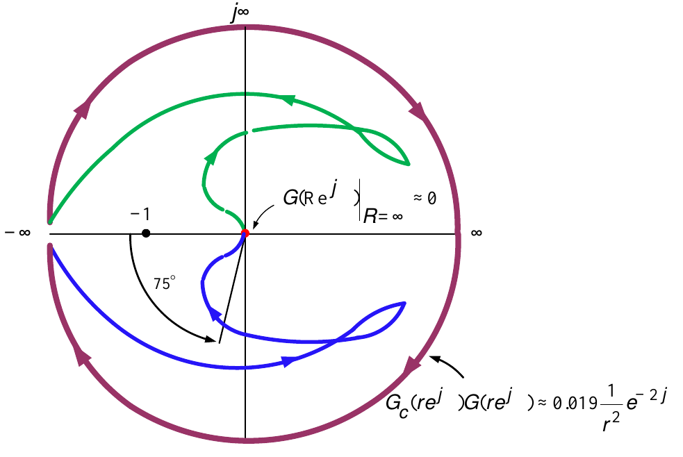
\(G_{c}(s)G(s)=\mathbf{K}(0.704s+1)\dfrac{s+0.1}{s}\dfrac{1.51s+0.1774}{s^{3}+0.739s^{2}+0.921s}\)
- Set \(K=5\) so \(20\log (5)=14\) dB
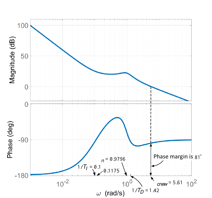
Gain crossover frequency is now \(\omega _{cnew}=5.61\) rad/sec.
The phase margin is now \(81^{\circ }.\)
\(G_{c}(s)=5(0.704s+1)\dfrac{s+0.1}{s}\)
(i.e., \(K=5\)).
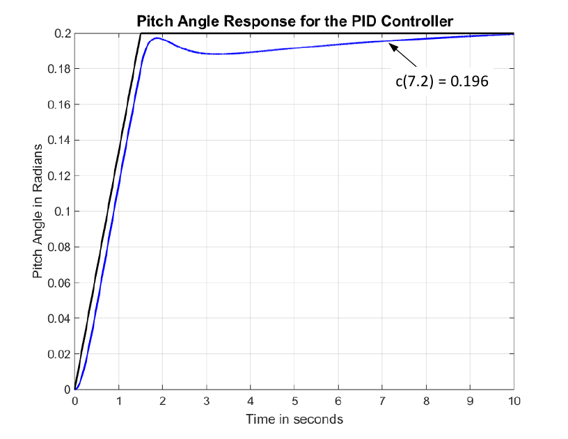
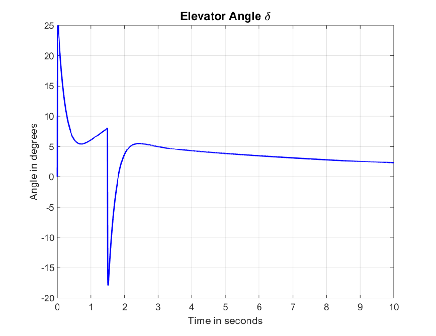
No overshoot, \(2\%\) settling time is \(t=7.2\) \(\sec\), rise time \(<2\sec\).