Pole Placement, 2-DoF Controllers, and Internal Stability

System Modeling and Control · Chapter 10

John N. Chiasson and Aykut C. Satici

Output Pole Placement
Two-Degree-of-Freedom Controllers
Internal Stability
Two-DOF Control of Aircraft Pitch

Pole Placement

The internal model principle:
- For tracking \(G_{c}(s)G(s)\) must contain the unstable poles of \(R(s).\)
- For disturbance rejection \(G_{c}(s)\) must contain the unstable poles of \(D(s).\)
- In either case, the closed-loop system must be stable.
The hard part is how to design \(G_{c}(s)\) to make the closed-loop system stable!
We now show how to find \(G_{c}(s)\) to place the CLPs at any desired location.

Example

Pole Placement for a Second-Order Control System

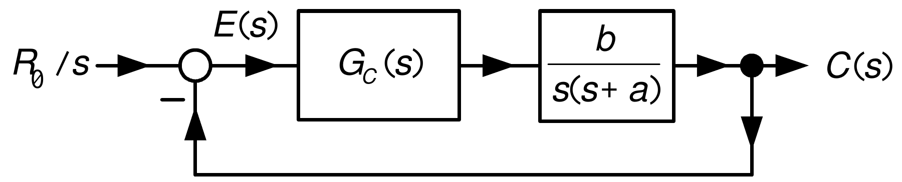
Objective: Track a step reference input.

The open-loop system is type 1.

\(G_{c}(s)\) must make the closed-loop system stable.

Let \(G_{c}(s)=\dfrac{b_{c}(s)}{a_{c}(s)}=\dfrac{b_{1}s+b_{0}}{s+a_{0}}.\)

\[ \begin{aligned} E(s)=\frac{1}{1+\dfrac{b_{1}s+b_{0}}{s+a_{0}}\dfrac{b}{s(s+a)}}\frac{R_{0} }{s} & =\frac{(s+a_{0})s(s+a)}{s(s+a)(s+a_{0})+(b_{1}s+b_{0})b}\frac{R_{0} }{s}\\ & =\frac{(s+a_{0})(s+a)}{s^{3}+\underset{f_{2}}{\underbrace{(a+a_{0})}} s^{2}+\underset{f_{1}}{\underbrace{(aa_{0}+bb_{1})}}s+\underset{f_{0} }{\underbrace{bb_{0}}}}R_{0}. \end{aligned} \]

\(s^{3}+f_{2}s^{2}+f_{1}s+f_{0}\) is the desired denominator of \(E(s).\)

Example

Pole Placement for a Second-Order Control System (continued)

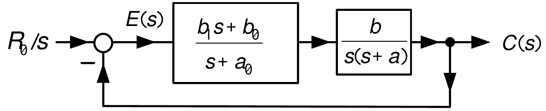
Set \(s^{3}+(a+a_{0})s^{2}+(aa_{0}+bb_{1})s+bb_{0}=s^{3}+f_{2}s^{2} +f_{1}s+f_{0}.\)

Equate powers of \(s\):

\[ \begin{aligned} bb_{0} & =f_{0}\\ aa_{0}+bb_{1} & =f_{1}\\ a+a_{0} & =f_{2} \end{aligned} \]

\[ \begin{aligned} b_{0} & =f_{0}/b\\ a_{0} & =f_{2}-a\\ b_{1} & =\frac{f_{1}-aa_{0}}{b}=\frac{f_{1}-af_{2}+a^{2}}{b}. \end{aligned} \]

Example

Pole Placement for a Second-Order Control System (continued)

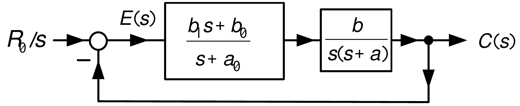
To put the closed-loop poles at \(-r_{1},-r_{2},-r_{3}\) set

\[ \begin{aligned} s^{3}+f_{2}s^{2}+f_{1}s+f_{0} & =(s+r_{1})(s+r_{2})(s+r_{3})\\ & \\ & =s^{3}+\underset{f_{2}}{\underbrace{(r_{1}+r_{2}+r_{3})}}s^{2} +\underset{f_{1}}{\underbrace{(r_{1}r_{2}+r_{1}r_{3}+r_{2}r_{3})} }s+\underset{f_{0}}{\underbrace{r_{1}r_{2}r_{3}}}. \end{aligned} \]

That is,

\[ \begin{aligned} f_{2} & =r_{1}+r_{2}+r_{3}\\ & \\ f_{1} & =r_{1}r_{2}+r_{1}r_{3}+r_{2}r_{3}\\ & \\ f_{0} & =r_{1}r_{2}r_{3}. \end{aligned} \]

Example

Disturbance Rejection for a Second-Order Control System

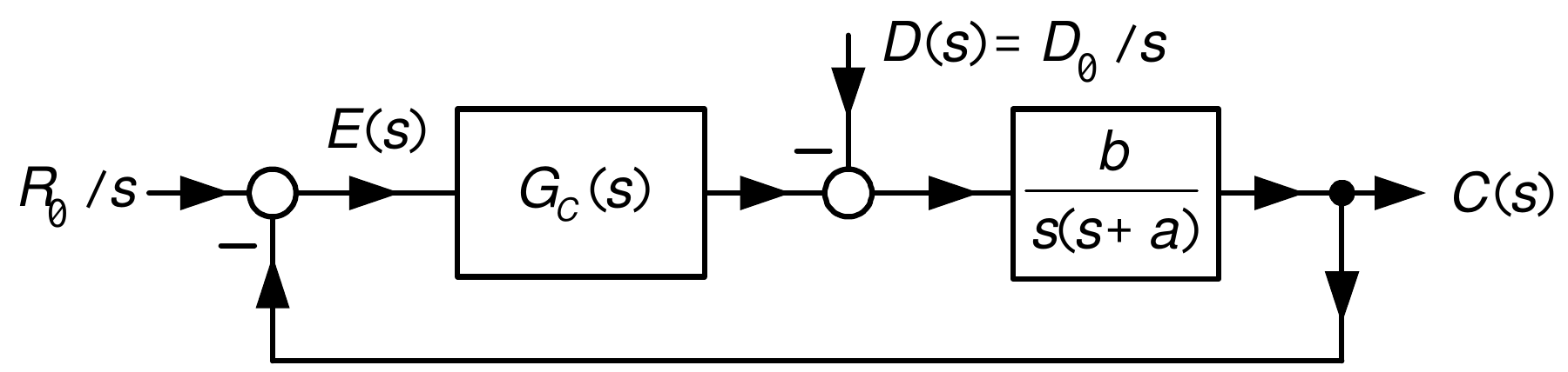
Set \(G_{c}(s)=\dfrac{b_{c}(s)}{a_{c}(s)}=\underset{\bar{G}_{c} (s)}{\underbrace{\dfrac{b_{2}s^{2}+b_{1}s+b_{0}}{s+a_{0}}}}\dfrac{1}{s}.\)

\(G_{c}(s)\) must have the factor \(1/s\) to satisfy the internal model principle.
The denominator of \(\bar{G}_{c}(s)\) has degree one less than the denominator of \(G(s).\)
The numerator of \(G_{c}(s)\) has the same degree as its denominator.

\[ \begin{aligned} E_{D}(s)=\frac{G(s)}{1+G_{c}(s)G(s)}\frac{D_{0}}{s} & =\frac{\dfrac {b}{s(s+a)}}{1+\dfrac{b_{2}s^{2}+b_{1}s+b_{0}}{s+a_{0}}\dfrac{1}{s}\dfrac {b}{s(s+a)}}\frac{D_{0}}{s}\\ & =\frac{s(s+a_{0})b}{s^{2}(s+a_{0})(s+a)+bb_{2}s^{2}+bb_{1}s+bb_{0}} \frac{D_{0}}{s}\\ & =\frac{(s+a_{0})b}{s^{4}+(a+a_{0})s^{3}+(aa_{0}+bb_{2})s^{2}+bb_{1}s+bb_{0} }D_{0}. \end{aligned} \]

Example

Disturbance Rejection for a Second-Order Control System (continued)

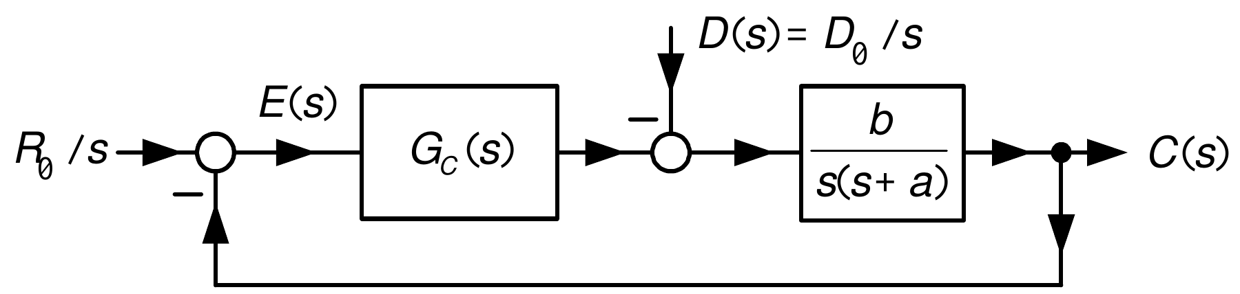
\(E_{D}(s)=\dfrac{(s+a_{0})b}{s^{4}+\underset{f_{3}}{\underbrace{(a+a_{0} )}}s^{3}+\underset{f_{2}}{\underbrace{(aa_{0}+bb_{2})}}s^{2}+\underset{f_{1} }{\underbrace{bb_{1}}}s+\underset{f_{0}}{\underbrace{bb_{0}}}}D_{0}.\)
\(s^{4}+f_{3}s^{3}+f_{2}s^{2}+f_{1}s+f_{0}\) is the desired denominator of \(E_{D}(s).\)
Solve \(s^{4}+(a+a_{0})s^{3}+(aa_{0}+bb_{2})s^{2}+bb_{1}s+bb_{0} =s^{4}+f_{3}s^{3}+f_{2}s^{2}+f_{1}s+f_{0}\):

\[ \begin{aligned} b_{0} & =f_{0}/b\\ b_{1} & =f_{1}/b\\ a_{0} & =f_{3}-a\\ b_{2} & =\frac{f_{2}-aa_{0}}{b}=\frac{f_{2}-af_{3}+a^{2}}{b}. \end{aligned} \]

Example

Tracking a Sinusoid

\(r(t)=R_{0}\sin(t)\) or \(R(s)=\dfrac{R_{0}}{s^{2}+1}\).

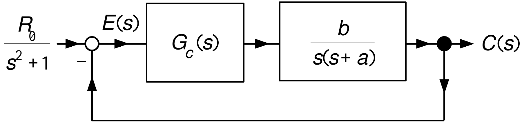
\(G_{c}(s)=\dfrac{b_{c}(s)}{a_{c}(s)}=\underset{\bar{G}_{c} (s)}{\underbrace{\dfrac{b_{3}s^{3}+b_{2}s^{2}+b_{1}s+b_{0}}{s+a_{0}}}} \dfrac{1}{s^{2}+1}.\)

\(G_{c}(s)\) must have factor \(\dfrac{1}{s^{2}+1}\) to satisfy the internal model principle.
The denominator of \(\bar{G}_{c}(s)\) has degree one less than the denominator of \(G(s).\)
The numerator of \(G_{c}(s)\) has the same degree as its denominator.

Example

Tracking a Sinusoid (continued)

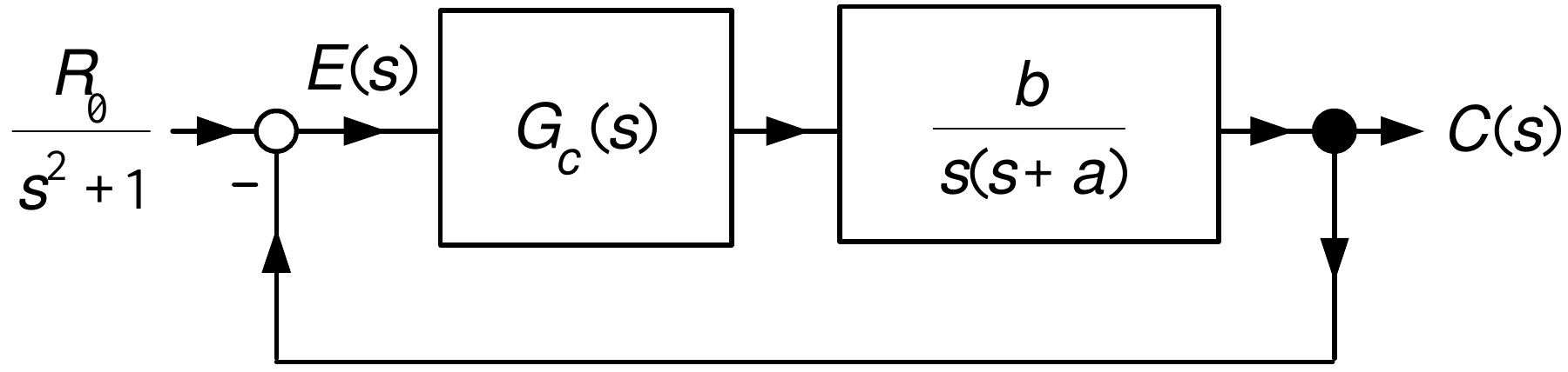
\[ \begin{aligned} \!\!\!\!\!E(s)\!\!\! & =\!\!\!\frac{1}{1+G_{c}(s)G(s)}R(s)\\ & \\ \!\!\! & =\!\!\!\frac{1}{1+\dfrac{b_{3}s^{3}+b_{2}s^{2}+b_{1}s+b_{0}} {s+a_{0}}\dfrac{1}{s^{2}+1}\dfrac{b}{s(s+a)}}\frac{R_{0}}{s^{2}+1}\\ & \\ \!\!\! & =\!\!\!\frac{(s+a_{0})s(s+a)(s^{2}+1)}{(s+a_{0})s(s+a)(s^{2} +1)+bb_{3}s^{3}+bb_{2}s^{2}+bb_{1}s+bb_{0}}\frac{R_{0}}{s^{2}+1}\\ & \\ \!\!\! & =\!\!\!\frac{(s+a_{0})s(s+a)}{s^{5}+(a+a_{0})s^{4}+(aa_{0} +bb_{3}+1)s^{3}+(a+a_{0}+bb_{2})s^{2}+(aa_{0}+bb_{1})s+bb_{0}}R_{0}. \end{aligned} \]

\(s^{5}+f_{4}s^{4}+f_{3}s^{3}+f_{2}s^{2}+f_{1}s+f_{0}\) is the desired denominator of \(E(s).\)

Example

Tracking a Sinusoid (continued)

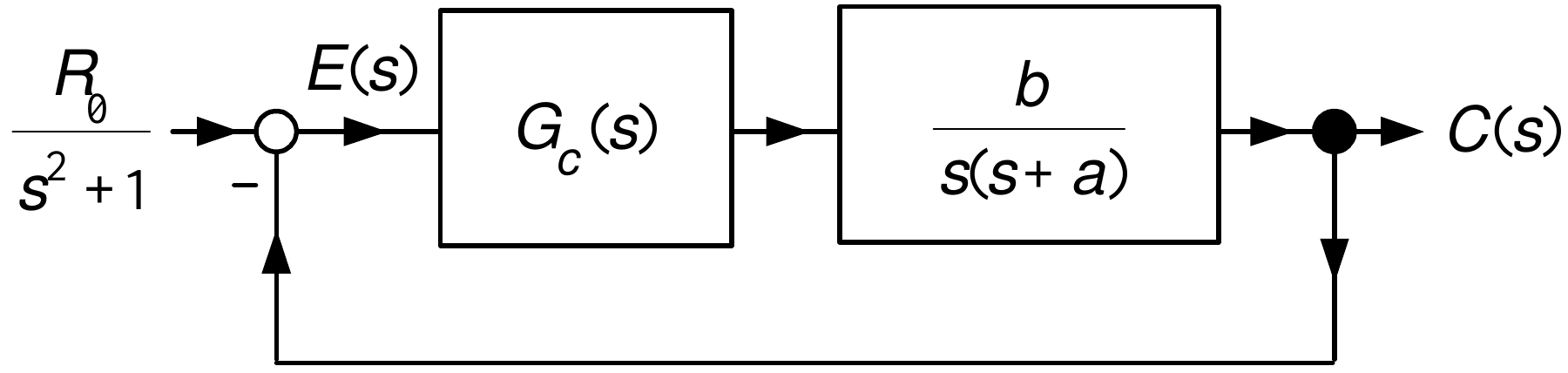
\[ \begin{aligned} & \!\!\!\!\!\!\!\!\!\!\!\!\!\!\!\!\!\!\!\!\!\!\!\!\!\!\!\!\!\!\!\!\!\!\!\!\!\!\!\!\!\!s^{5} +(a+a_{0})s^{4}+(aa_{0}+bb_{3}+1)s^{3}+(a+a_{0}+bb_{2})s^{2}+(aa_{0} +bb_{1})s+bb_{0}\\ & \\ & \quad\qquad\qquad=\quad s^{5}+f_{4}s^{4}+f_{3}s^{3}+f_{2}s^{2}+f_{1}s+f_{0}. \end{aligned} \]

This requires setting

\[ \begin{aligned} b_{0} & =\frac{f_{0}}{b}\\ a_{0} & =f_{4}-a\\ b_{1} & =\frac{f_{1}-aa_{0}}{b}=\frac{f_{1}-af_{4}+a^{2}}{b}\\ b_{2} & =\frac{f_{2}-a-a_{0}}{b}=\frac{f_{2}-f_{4}}{b}\\ b_{3} & =\frac{f_{3}-aa_{0}-1}{b}=\frac{f_{3}-af_{4}+a^{2}+1}{b}. \end{aligned} \]

Example

Pole Placement

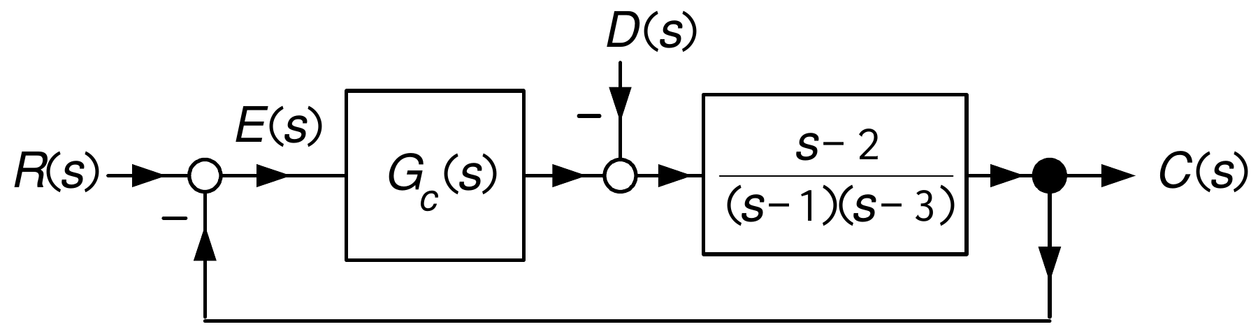
\(R(s)=\dfrac{R_{0}}{s},D(s)=\dfrac{D_{0}}{s}\) and \(G_{c}(s)=\underset{\bar {G}_{c}(s)}{\underbrace{\dfrac{b_{2}s^{2}+b_{1}s+b_{0}}{s+a_{0}}}}\dfrac{1} {s}.\)

\(G_{c}(s)\) must have factor \(\dfrac{1}{s}\) to satisfy the internal model principle.
The denominator of \(\bar{G}_{c}(s)\) has degree one less than the denominator of \(G(s).\)
The numerator of \(G_{c}(s)\) has the same degree as its denominator.

\[ \begin{aligned} \!\!\!E_{R}(s)=\frac{1}{1+G_{c}(s)G(s)}R(s) & =\!\!\!\frac{1}{1+\dfrac {b_{2}s^{2}+b_{1}s+b_{0}}{s+a_{0}}\dfrac{1}{s}\dfrac{s-2}{(s-1)(s-3)}} \frac{R_{0}}{s}\\ & \\ & =\!\!\!\frac{s(s+a_{0})(s-1)(s-3)}{s(s+a_{0})(s-1)(s-3)+(b_{2}s^{2} +b_{1}s+b_{0})(s-2)}\frac{R_{0}}{s}. \end{aligned} \]

Example

Pole Placement (continued)

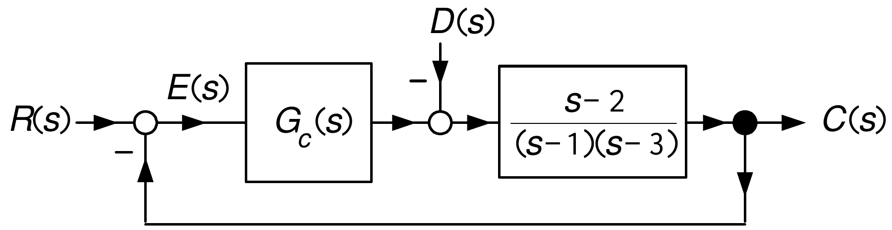
\[ \begin{aligned} E_{R}(s) & =\frac{s(s+a_{0})(s-1)(s-3)}{s(s+a_{0})(s-1)(s-3)+(b_{2} s^{2}+b_{1}s+b_{0})(s-2)}\frac{R_{0}}{s}\\ & \\ & =\frac{(s+a_{0})(s-1)(s-3)}{s^{4}+(b_{2}+a_{0}-4)s^{3}+(b_{1}-2b_{2} -4a_{0}+3)s^{2}+(3a_{0}+b_{0}-2b_{1})s-2b_{0}}R_{0}. \end{aligned} \]

Set

\[ s^{4}+(b_{2}+a_{0}-4)s^{3}+(b_{1}-2b_{2}-4a_{0}+3)s^{2}+(3a_{0}+b_{0} -2b_{1})s-2b_{0}= \]

\(\quad\quad\quad\!\!\!s^{4}+f_{3}s^{3}+f_{2}s^{2}+f_{1}s+f_{0}.\)

In matrix form: \(\left[ \begin{array}{c} f_{3}\\ f_{2}\\ f_{1}\\ f_{0} \end{array} \right] =\left[ \begin{array}{rrrr} 1 & 0 & 0 & 1\\ -2 & 1 & 0 & -4\\ 0 & -2 & 1 & 3\\ 0 & 0 & -2 & 0 \end{array} \right] \!\left[ \begin{array}{c} b_{2}\\ b_{1}\\ b_{0}\\ a_{0} \end{array} \right] +\left[ \begin{array}{r} -4\\ 3\\ 0\\ 0 \end{array} \right] .\)

Example

Pole Placement (continued)

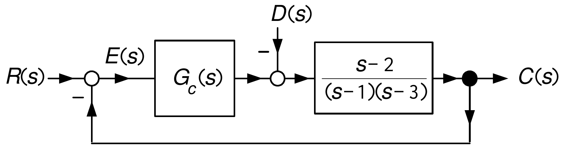
Solve to obtain

\[ \begin{aligned} \left[ \begin{array}{c} b_{2}\\ b_{1}\\ b_{0}\\ a_{0} \end{array} \right] & =\left[ \begin{array}{rrrr} 1 & 0 & 0 & 1\\ -2 & 1 & 0 & -4\\ 0 & -2 & 1 & 3\\ 0 & 0 & -2 & 0 \end{array} \right] ^{-1}\left( \left[ \begin{array}{c} f_{3}\\ f_{2}\\ f_{1}\\ f_{0} \end{array} \right] -\left[ \begin{array}{r} -4\\ 3\\ 0\\ 0 \end{array} \right] \right) \\ & =\left[ \begin{array}{rrrr} 5 & 2 & 1 & 1/2\\ -6 & -3 & -2 & -1\\ 0 & 0 & 0 & -1/2\\ -4 & -2 & -1 & -1/2 \end{array} \right] \left( \left[ \begin{array}{c} f_{3}\\ f_{2}\\ f_{1}\\ f_{0} \end{array} \right] -\left[ \begin{array}{r} -4\\ 3\\ 0\\ 0 \end{array} \right] \right) \\ & =\left[ \begin{array}{l} f_{0}/2+f_{1}+2f_{2}+5f_{3}+14\\ -f_{0}-2f_{1}-3f_{2}-6f_{3}-15\\ -f_{0}/2\\ -f_{0}/2-f_{1}-2f_{2}-4f_{3}-10 \end{array} \right] . \end{aligned} \]

Example

Pole Placement (continued)

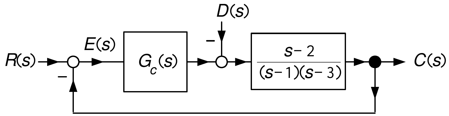
To put the closed-loop poles at \(-r_{1},-r_{2},-r_{3},-r_{4}\) we simply set

\[ \begin{aligned} s^{4}+f_{3}s^{3}+f_{2}s^{2}+f_{1}s+f_{0} & =(s+r_{1})(s+r_{2})(s+r_{3} )(s+r_{4})\\ & \\ & =s^{4}+\underset{f_{3}}{\underbrace{(r_{1}+r_{2}+r_{3}+r_{4})}}s^{3}+\\ & \underset{f_{2}}{\underbrace{(r_{1}r_{2}+r_{1}r_{3}+r_{1}r_{4}+r_{2} r_{3}+r_{2}r_{4}+r_{3}r_{4})}}s^{2}+\\ & \underset{f_{1}}{\underbrace{\left( r_{1}r_{2}r_{3}+r_{1}r_{2}r_{4} +r_{1}r_{3}r_{4}+r_{2}r_{3}r_{4}\right) }}s+\underset{f_{0} }{\underbrace{r_{1}r_{2}r_{3}r_{4}}} \end{aligned} \]

Example

Pole Placement (continued)

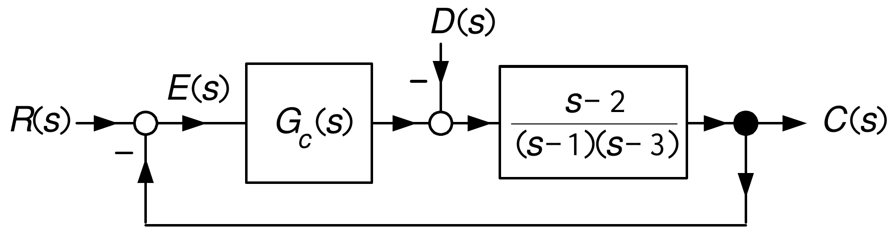
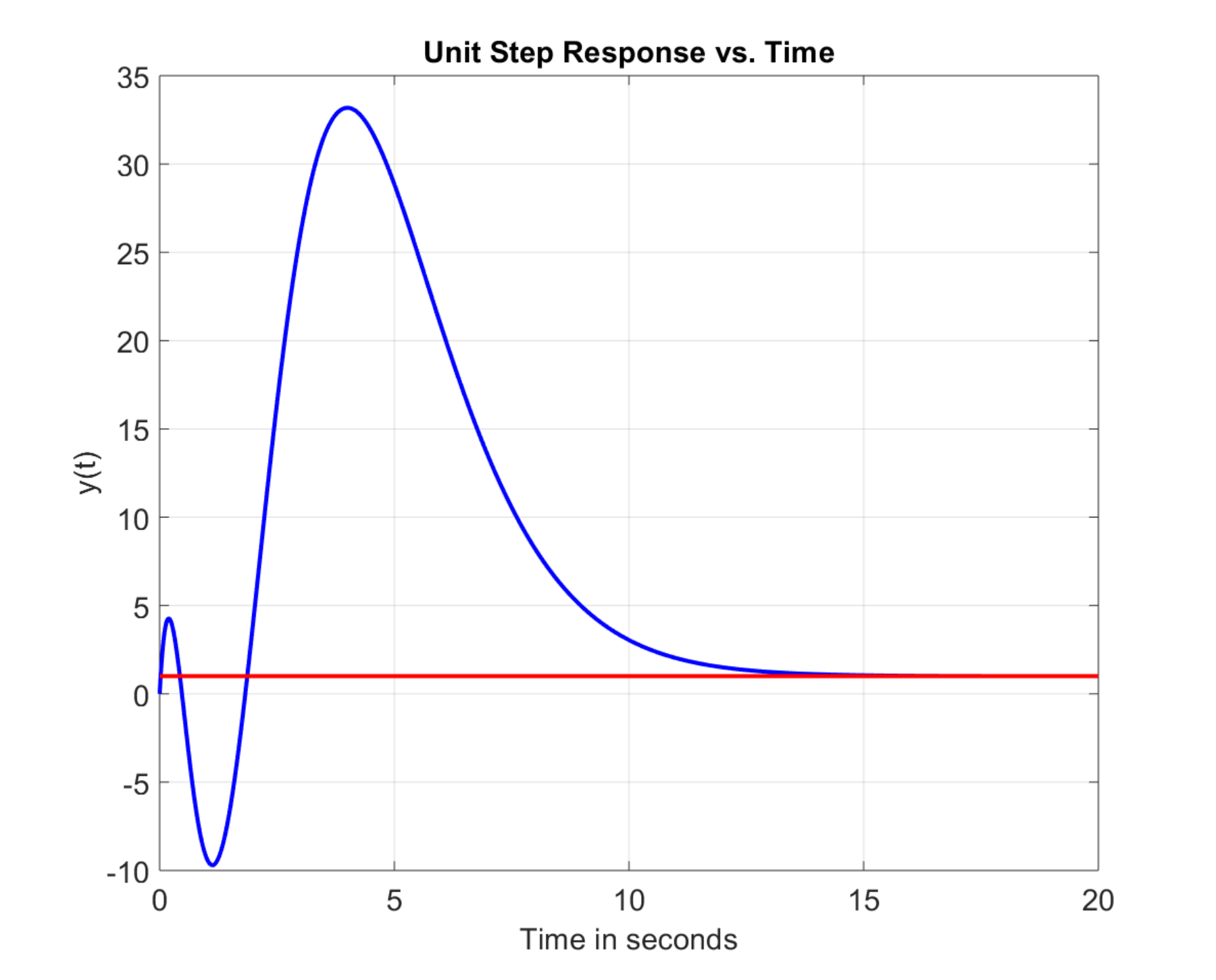
\(\!\!\!\!\!\!\)Closed-loop response \(C_{R}(s)=\dfrac{G_{c} (s)G(s)}{1+G_{c}(s)G(s)}R(s).\)

Let \(R(s)=1/s\) with the closed-loop poles placed at \(-1.\)

Too much overshoot in the step response!

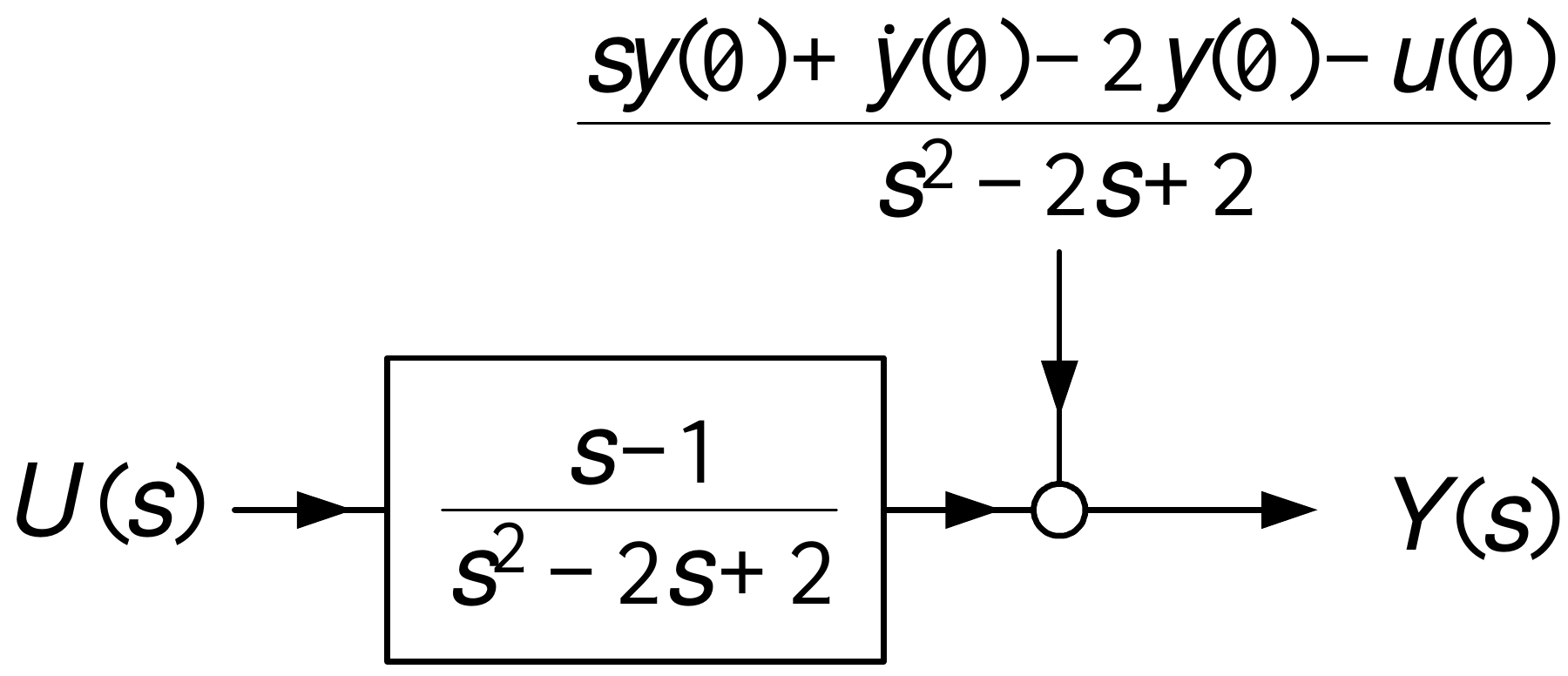
Effect of the Initial Conditions on the Control Design

We have always taken the initial conditions to be zero!
What happens if they are not zero?

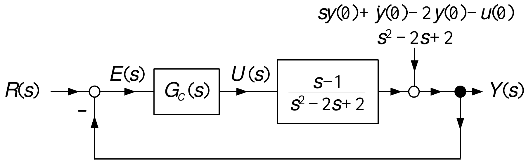
Consider

\[ \ddot{y}-2\dot{y}+2y=\dot{u}-u \]

where

\[ s^{2}Y(s)-sy(0)-\dot{y}(0)-2sY(s)+2y(0)+2Y(s)=sU(s)-u(0)-U(s) \]

\[ Y(s)=\underset{G(s)}{\underbrace{\frac{s-1}{s^{2}-2s+2}}}U(s)+\frac {sy(0)+\dot{y}(0)-2y(0)-u(0)}{s^{2}-2s+2}. \]

Key observation

\(G(s)\) and the initial condition term always have the same denominator.

Effect of the Initial Conditions on the Control Design

Let \(G_{c}(s)=\dfrac{-2s+13}{s+7}\) to put all 3 closed-loop poles at \(-1.\)

\[ \begin{aligned} Y(s) & =G(s)U(s)+\frac{sy(0)+\dot{y}(0)-2y(0)-u(0)}{s^{2}-2s+2}\\ & \\ & =G(s)G_{c}(s)\!\left( R(s)-Y(s)\right) +\frac{sy(0)+\dot {y}(0)-2y(0)-u(0)}{s^{2}-2s+2} \end{aligned} \]

\[ \begin{aligned} & \Longrightarrow\left( 1+G(s)G_{c}(s)\right) \!\!Y(s)=G(s)G_{c}(s)R(s)+\frac{sy(0)+\dot{y}(0)-2y(0)-u(0)}{s^{2}-2s+2}\\ & \\ & \Longrightarrow Y(s)=\frac{G(s)G_{c}(s)}{1+G(s)G_{c}(s)} R(s)+\underset{Y_{IC}(s)}{\underbrace{\frac{1}{1+G(s)G_{c}(s)}\frac {sy(0)+\dot{y}(0)-2y(0)-u(0)}{s^{2}-2s+2}}}. \end{aligned} \]

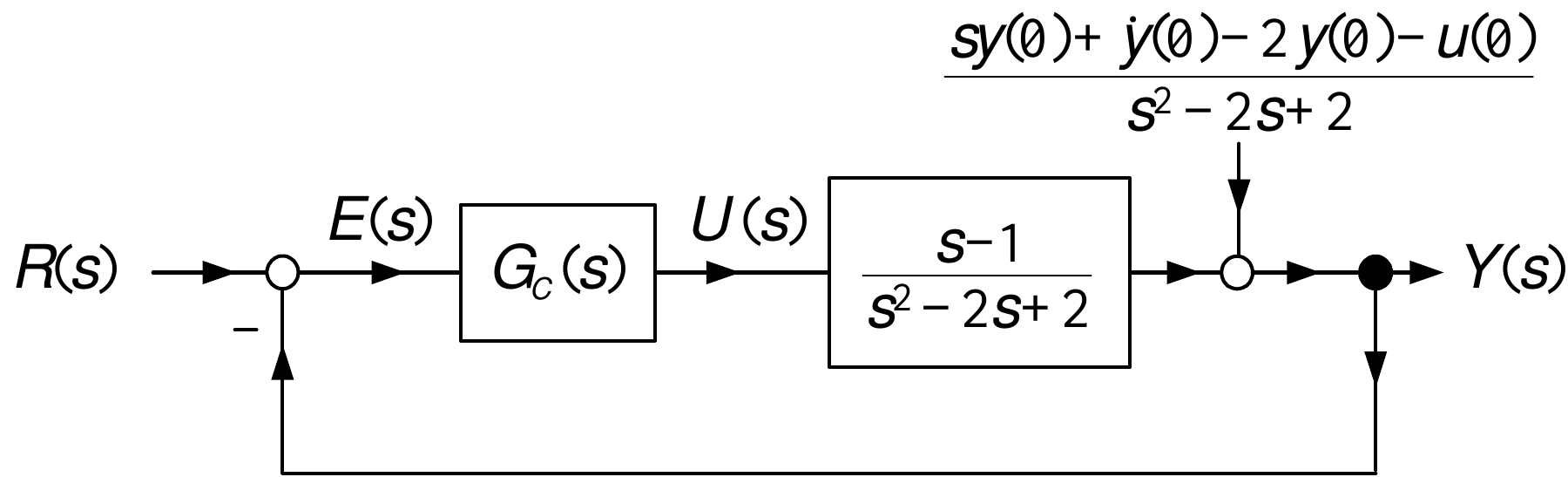
Effect of the Initial Conditions on the Control Design

As \(G_{c}(s)=\dfrac{-2s+13}{s+7}\), the initial condition response \(Y_{IC}(s)\) simplifies to

\[ \begin{aligned} Y_{IC}(s) & \triangleq\frac{1}{1+\dfrac{s-1}{s^{2}-2s+2}\dfrac{-2s+13}{s+7} }\frac{sy(0)+\dot{y}(0)-2y(0)-u(0)}{s^{2}-2s+2}\\ & \\ & \\ & =\frac{(s^{2}-2s+2)(s+7)}{s^{3}+3s^{2}+3s+1}\frac{sy(0)+\dot{y} (0)-2y(0)-u(0)}{s^{2}-2s+2}\\ & \\ & \\ & =\frac{(s+7)(sy(0)+\dot{y}(0)-2y(0)-u(0))}{(s+1)(s+1)(s+1)}. \end{aligned} \]

Effect of the Initial Conditions on the Control Design

\[ y_{IC}(t)=\mathcal{L}^{-1}\{Y_{IC}(s)\}=\mathcal{L}^{-1}\left\{ \frac{(s+7)(sy(0)+\dot{y}(0)-2y(0)-u(0))}{(s+1)(s+1)(s+1)} \right\} \rightarrow0. \]

\[ \begin{aligned} Y_{R}(s)=\underset{G_{CL}(s)}{\underbrace{\frac{G(s)G_{c}(s)}{1+G(s)G_{c}(s)} }}R(s) & =\frac{\dfrac{s-1}{s^{2}-2s+2}\dfrac{-2s+13}{s+7}}{1+\dfrac {s-1}{s^{2}-2s+2}\dfrac{-2s+13}{s+7}}R(s)\\ & =\frac{(s-1)(-2s+13)}{s^{3}+3s^{2}+3s+1}R(s)\\ & =\frac{(s-1)(-2s+13)}{(s+1)(s+1)(s+1)}R(s) \end{aligned} \]

\(Y_{IC}(s)\) and \(Y_{R}(s)/R(s)=G_{CL}(s)\) always have the same denominator.
As long as the closed-loop system is stable, the initial condition response asymptotically goes to zero.

Example

Inverted Pendulum

The center of mass of the rod is at \((x+\ell\sin(\theta ),y)\approx(x+\ell\theta,y)\) for \(\theta\) small.
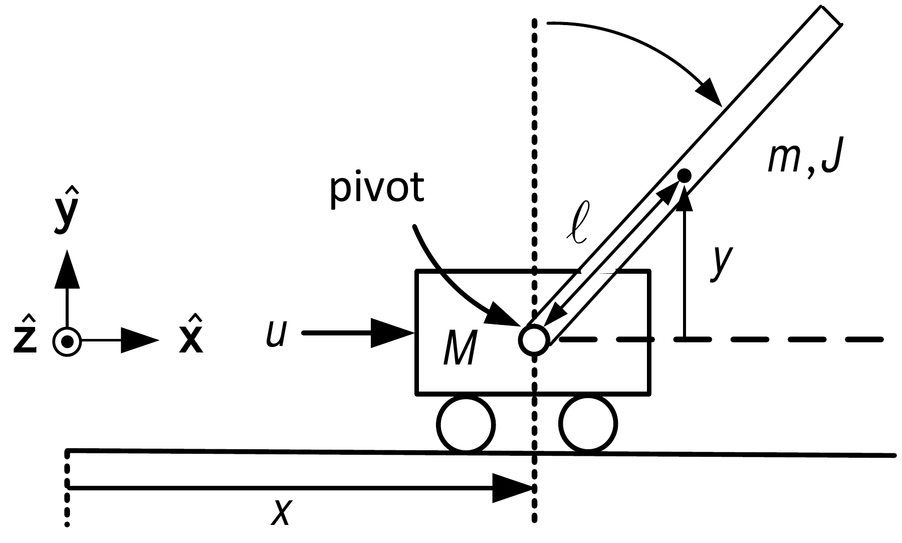
With an abuse of notation we also let \(y\triangleq x+\left( \ell +\dfrac{J}{m\ell}\right) \theta.\)
Then

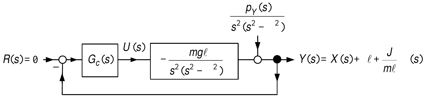
\[ Y(s)=X(s)+\left( \ell+\frac{J}{m\ell}\right) \theta(s)=\text{ } \underset{G_{Y}(s)}{\underbrace{-\kappa\frac{mg\ell}{s^{2}(s^{2}-\alpha^{2})} }}U(s)+\frac{p_{Y}(s)}{s^{2}(s^{2}-\alpha^{2})} \]

where

\[ \begin{aligned} p_{Y}(s) & \triangleq(J/(m\ell)+\ell)s^{2}-\kappa g(m\ell)^{2})(s\theta (0)+\dot{\theta}(0))+(s^{2}-\alpha^{2})(sx(0)+\dot{x}(0)),\\ \alpha^{2} & =\frac{mg\ell(M+m)}{Mm\ell^{2}+J(M+m)},\\ \kappa & =\frac{1}{Mm\ell^{2}+J(M+m)}. \end{aligned} \]

Example

Inverted Pendulum (continued)

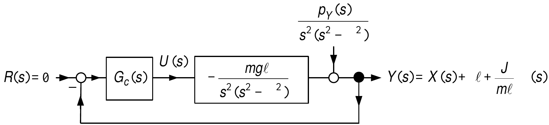
Stabilize \(y\triangleq x+\left( \ell+\dfrac{J}{m\ell}\right) \theta\rightarrow0.\)
Find \(G_{c}(s)=\dfrac{b_{c}(s)}{a_{c}(s)}\) so \(U(s)=-G_{c}(s)Y(s)\) stabilizes the pendulum to \(y=0\).
This linear model is only valid for \((x,\dot{x},\theta ,\dot{\theta})\) close to \((0,0,0,0).\)

\(\qquad\Longrightarrow\) \(\ \ (x(0),\dot{x}(0),\theta(0),\dot{\theta}(0))\) must be close to \((0,0,0,0)\).
With \(U(s)=-G_{c}(s)Y(s)\) we have

\[ Y(s)=-G_{Y}(s)G_{c}(s)Y(s)+\frac{p(s)}{s^{2}(s^{2}-\alpha^{2})}. \]

Example

Inverted Pendulum (continued)

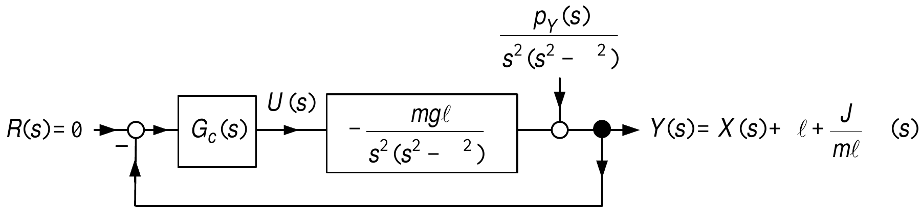
Previous slide:

\[ Y(s)=-G_{Y}(s)G_{c}(s)Y(s)+\frac{p_{Y}(s)}{s^{2}(s^{2}-\alpha^{2})}. \]

Solve for \(Y(s)\) to obtain

\[ \begin{aligned} Y(s) & =\frac{1}{1+G_{Y}(s)G_{c}(s)}\frac{p_{Y}(s)}{s^{2}(s^{2}-\alpha^{2} )}\\ & =\frac{1}{1+\dfrac{b_{3}s^{3}+b_{2}s^{2}+b_{1}s+b_{0}}{s^{3}+a_{2} s^{2}+a_{1}s+a_{0}}\dfrac{-\kappa mg\ell}{s^{2}(s^{2}-\alpha^{2})}}\frac {p_{Y}(s)}{s^{2}(s^{2}-\alpha^{2})}\\ & =\frac{(s^{3}+a_{2}s^{2}+a_{1}s+a_{0})p_{Y}(s)}{(s^{3}+a_{2}s^{2} +a_{1}s+a_{0})s^{2}(s^{2}-\alpha^{2})+\left( -\kappa mg\ell\right) (b_{3}s^{3}+b_{2}s^{2}+b_{1}s+b_{0})}. \end{aligned} \]

Example

Inverted Pendulum (continued)

Collecting terms in \(s\) the denominator of \(Y(s)\) is rewritten as

\[ \begin{aligned} & \!\!\!\!\!\!\!\!\!\!\!\!\!\!\!\!\!\!\!\!\!\!\!\!\!\!\!\!\!\!\!\!\!\!\!\!\!s^{7} +a_{2}s^{6}+\left( a_{1}-\alpha^{2}\right) s^{5}+\left( a_{0}-\alpha ^{2}a_{2}\right) s^{4}+\left( -a_{1}\alpha^{2}-\kappa mg\ell b_{3}\right) s^{3}+\\ & \left( -a_{0}\alpha^{2}-\kappa mg\ell b_{2}\right) s^{2}-\kappa mg\ell b_{1}s-\kappa mg\ell b_{0} \end{aligned} \]

Let the desired denominator polynomial of \(Y(s)\) be

\[ s^{7}+f_{6}s^{6}+f_{5}s^{5}+f_{4}s^{4}+f_{3}s^{3}+f_{2}s^{2}+f_{1}s+f_{0}. \]

Set

\[ \begin{aligned} -\kappa mg\ell b_{0} & =f_{0}\\ -\kappa mg\ell b_{1} & =f_{1}\\ -a_{0}\alpha^{2}-\kappa mg\ell b_{2} & =f_{2}\\ -a_{1}\alpha^{2}-\kappa mg\ell b_{3} & =f_{3}\\ a_{0}-a_{2}\alpha^{2} & =f_{4}\\ a_{1}-\alpha^{2} & =f_{5}\\ a_{2} & =f_{6} \end{aligned} \]

Example

Inverted Pendulum (continued)

In matrix form we have

\[ \left[ \begin{array}{ccccccc} -\kappa mg\ell & 0 & 0 & 0 & 0 & 0 & 0\\ 0 & -\kappa mg\ell & 0 & 0 & 0 & 0 & 0\\ 0 & 0 & -\kappa mg\ell & 0 & -\alpha^{2} & 0 & 0\\ 0 & 0 & 0 & -\kappa mg\ell & 0 & -\alpha^{2} & 0\\ 0 & 0 & 0 & 0 & 1 & 0 & -\alpha^{2}\\ 0 & 0 & 0 & 0 & 0 & 1 & 0\\ 0 & 0 & 0 & 0 & 0 & 0 & 1 \end{array} \right] \left[ \begin{array}{c} b_{0}\\ b_{1}\\ b_{2}\\ b_{3}\\ a_{0}\\ a_{1}\\ a_{2} \end{array} \right] =\left[ \begin{array}{c} f_{0}\\ f_{1}\\ f_{2}\\ f_{3}\\ f_{4}\\ f_{5}+\alpha^{2}\\ f_{6} \end{array} \right] . \]

This matrix is invertible so we can solve for \(a_{0},a_{1},a_{2},b_{0} ,b_{1},b_{2},b_{3}.\)

Example

Inverted Pendulum (continued)

Quanser inverted pendulum: \(\kappa mg\ell=36.5705,\alpha^{2}=29.256\) so

\[ G_{Y}(s)=\frac{-36.5705}{s^{2}(s^{2}-29.256)}=\frac{-36.5705}{s^{2} (s+5.4089)(s-5.4089)}. \]

Choosing the seven closed-loop poles to be at \(-5\) results in

\[ \begin{aligned} G_{c}(s) & =-\frac{1041.6s^{3}+6113.7s^{2}+2990.8s+2136.3}{s^{3} +35s^{2}+554.3s+5399}\\ & \\ & =-\frac{1041.6(s+5.4088)(s^{2}+0.4308s+0.3792)}{(s+20.833)(s^{2} +14.1672s+259.1533)}. \end{aligned} \]

This controller has small stability margins making it very sensitve to disturbances.
- Small disturbances can cause \(\theta(t)\) to go far from \(0.\)
- \(G_{Y}(s)\) is then no longer a valid approximation of the nonlinear IP model.
- \(G_{c}(s)\) will not be able to bring \(\theta(t)\) back to \(0.\)

Example

Two Degrees of Freedom (2 DOF) Controllers

A PI controller typically results in the closed-loop TF having a left half-plane zero.
Zeros can cause or increase the amount of overshoot.
A two degrees of freedom controller can often be used to eliminate overshoot.

Two Degrees of Freedom Controllers

Consider the PID control system.

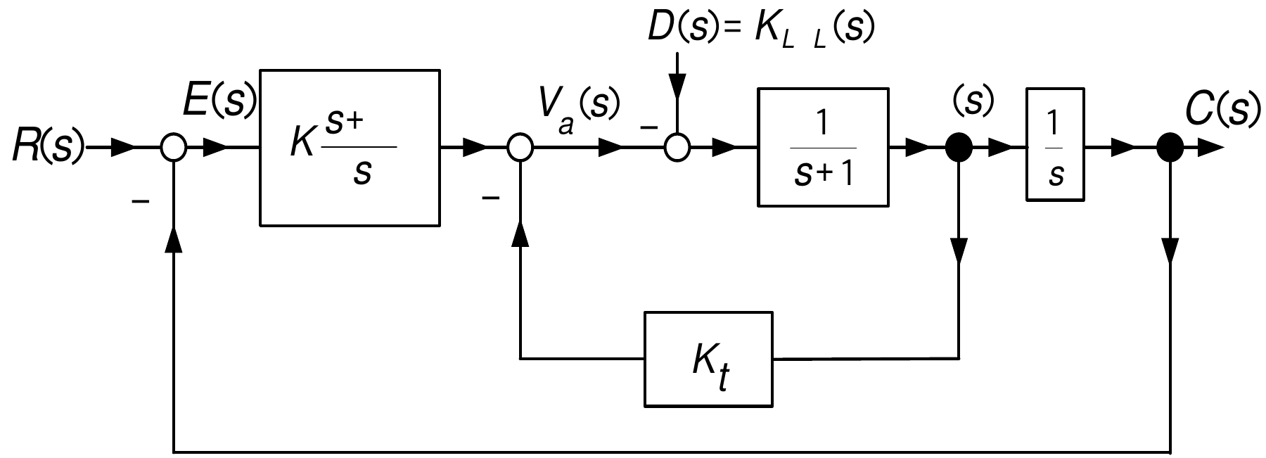
Block diagram reduction:

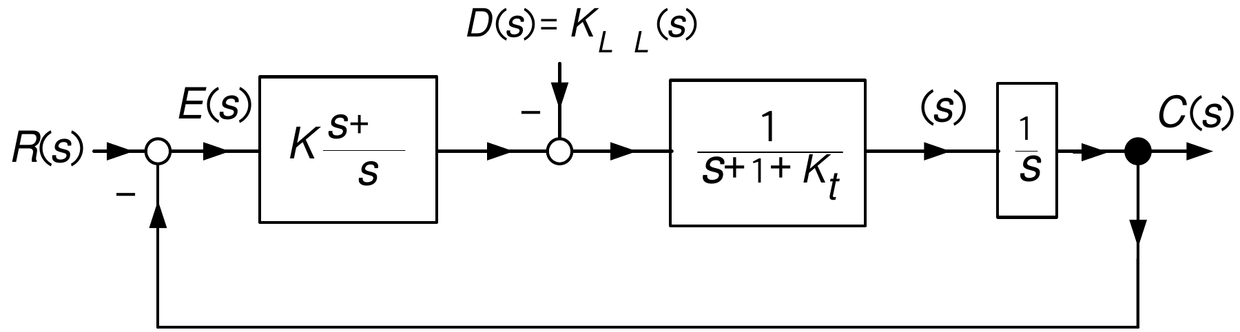
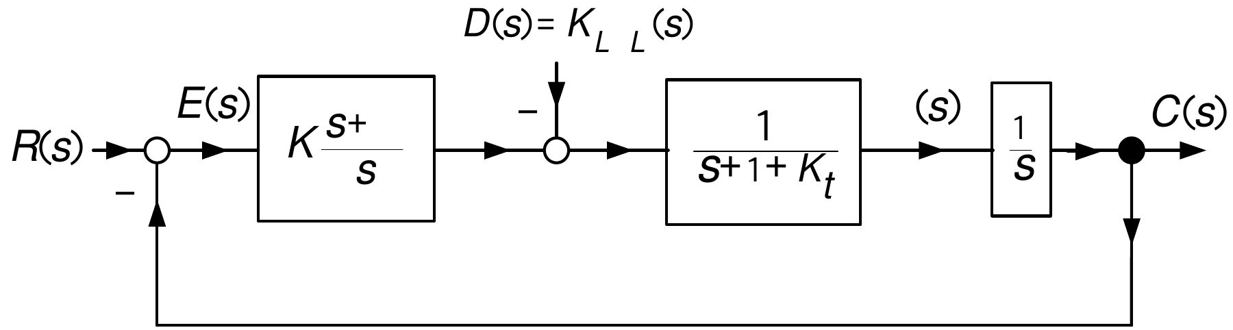
Two Degrees of Freedom Controllers

Let’s first look at making the closed-loop system stable.

\[ E_{R}(s)=\frac{1}{1+K\dfrac{s+\alpha}{s}\dfrac{1}{s+1+K_{t}}\dfrac{1}{s} }R(s)=\frac{s^{2}(s+1+K_{t})}{s^{3}+(1+K_{t})s^{2}+Ks+\alpha K}R(s) \]

Choose the closed-loop poles to be \(-r_{1},-r_{2},-r_{3}\) with \(r_{1}>0,r_{2}>0,r_{3}>0.\)

\[ \begin{aligned} s^{3}+(1+K_{t})s^{2}+Ks+\alpha K\!\!\! & =\!\!\!(s+r_{1})(s+r_{2})(s+r_{3})\\ \!\!\! & =\!\!\!s^{3}+(r_{1}+r_{2}+r_{3})s^{2}+(r_{1}r_{2}+r_{1}r_{3} +r_{2}r_{3})s+r_{1}r_{2}r_{3}. \end{aligned} \]

\[ \Longrightarrow\quad{}K_{t}=r_{1}+r_{2}+r_{3}-1,\quad{}K=r_{1} r_{2}+r_{1}r_{3}+r_{2}r_{3},\text{ }\alpha=\frac{r_{1}r_{2}r_{3}}{K} =\frac{r_{1}r_{2}r_{3}}{r_{1}r_{2}+r_{1}r_{3}+r_{2}r_{3}}. \]

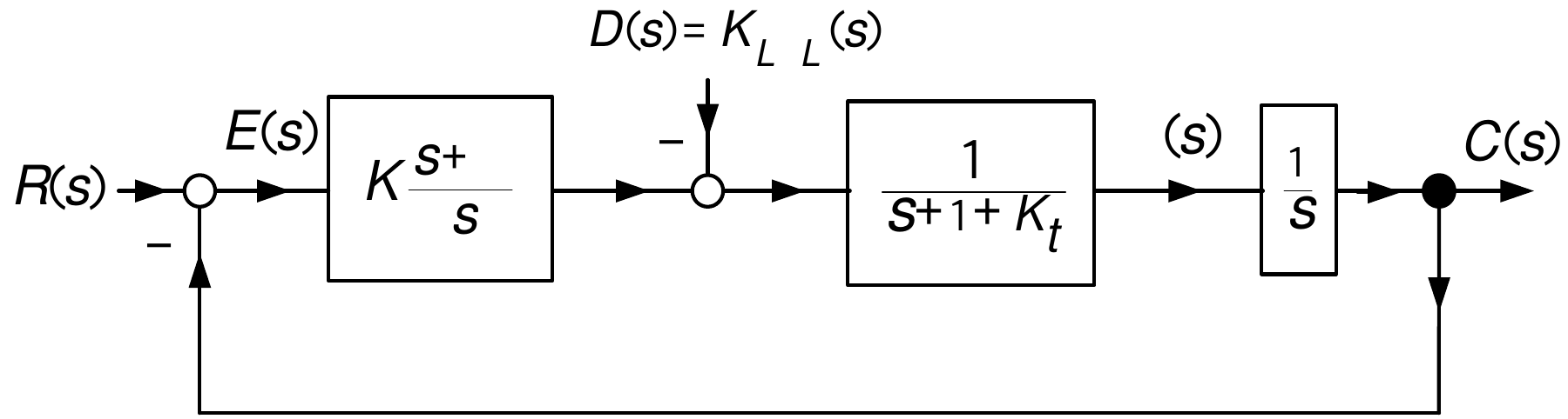
Two Degrees of Freedom Controllers

\[ \begin{aligned} C_{R}(s)=\frac{K\dfrac{s+\alpha}{s}\dfrac{1}{s+1+K_{t}}\dfrac{1}{s}} {1+K\dfrac{s+\alpha}{s}\dfrac{1}{s+1+K_{t}}\dfrac{1}{s}}\frac{R_{0}}{s} & =\frac{K(s+\alpha)}{s^{3}+(1+K_{t})s^{2}+Ks+\alpha K}\frac{R_{0}}{s}\\ & =\frac{K(s+\alpha)}{(s+r_{1})(s+r_{2})(s+r_{3})}\frac{R_{0}}{s}. \end{aligned} \]

\(sC_{R}(s)\) is stable so by the FVT

\[ c_{R}(\infty)=\lim_{s\rightarrow0}sC_{R}(s)=\lim_{s\rightarrow0} s\frac{K(s+\alpha)}{s^{3}+(1+K_{t})s^{2}+Ks+\alpha K}\frac{R_{0}}{s}=R_{0}. \]

Problem: \(c_{R}(t)\) will exhibit overshoot.

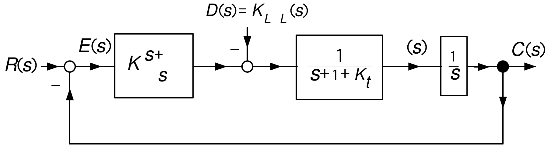
Two Degrees of Freedom Controllers

\[ C_{R}(s)=\frac{K\dfrac{s+\alpha}{s}\dfrac{1}{s+1+K_{t}}\dfrac{1}{s}} {1+K\dfrac{s+\alpha}{s}\dfrac{1}{s+1+K_{t}}\dfrac{1}{s}}\frac{R_{0}}{s} =\frac{K(s+\alpha)}{(s+r_{1})(s+r_{2})(s+r_{3})}\frac{R_{0}}{s}. \]

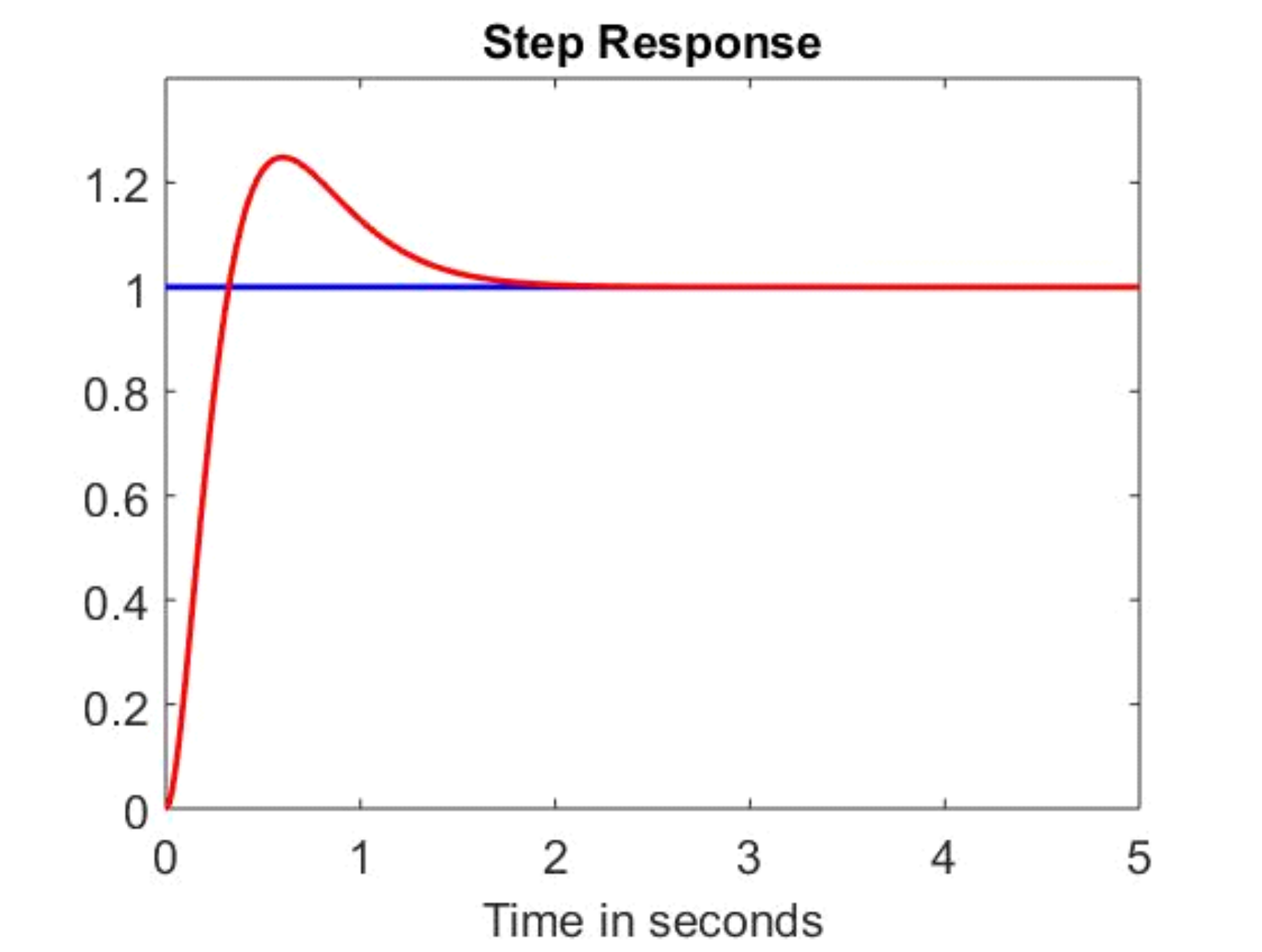
With this control architecture, there will always be overshoot as we explain next.

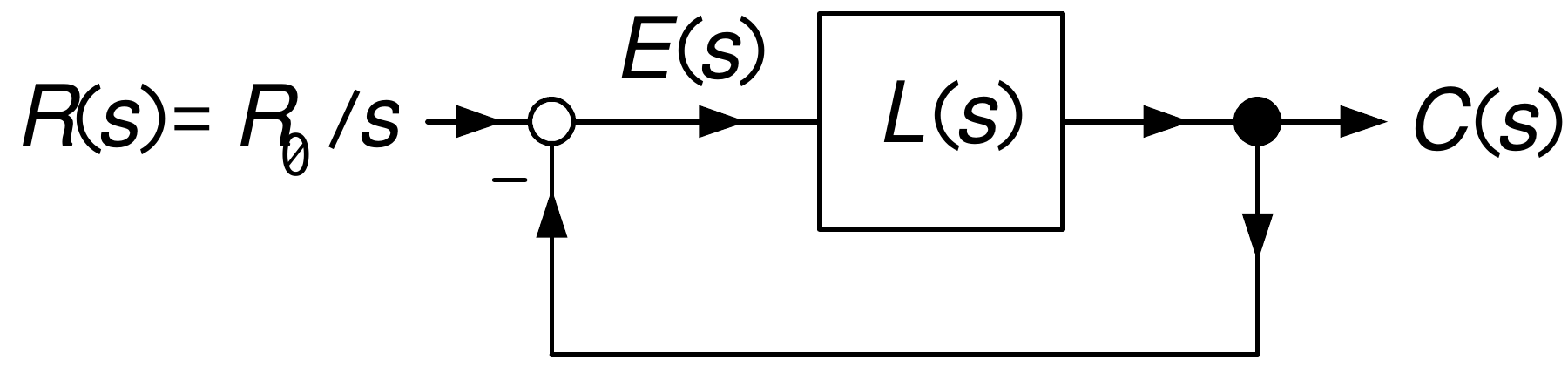
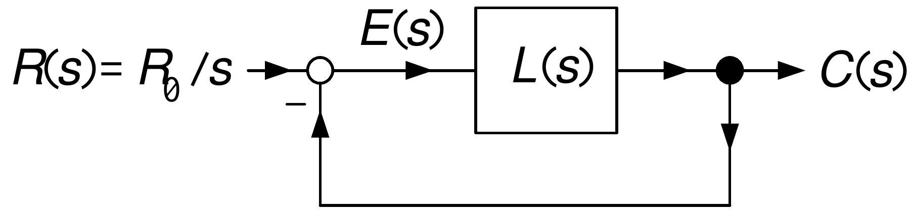
Stable Type 2 Systems Have Overshoot

\(L(s)\triangleq K\dfrac{s+\alpha}{s}\dfrac{1}{s+1+K_{t}}\dfrac{1}{s}\) is a type 2 system.
The closed-loop system is \(G_{CL}(s)=\dfrac{L(s)}{1+L(s)}\) is stable.
We chose the gains \(\alpha,K,K_{t}\) to put the poles at \(-r_{1} ,-r_{2},-r_{3}.\)

Theorem Stable Type 2 Systems Have Overshoot

The step response of any stable type 2 system has overshoot.

Proof: See Appendix.

Stable Systems with Real Poles and No Zeros Do Not Have Overshoot

Theorem Stable Systems with Real Poles and No Zeros Do Not Have Overshoot

Let a system satisfy the following conditions:

(1) The closed-loop transfer function is stable.

(2) The closed-loop transfer function has real poles.

(3) The closed-loop transfer function has no zeros.

Then its step response has no overshoot.

Proof: See Appendix.

Stable Systems with Real Poles and No Zeros Do Not Have Overshoot

\[ C_{R}(s)=\frac{K(s+\alpha)}{s^{3}+(1+K_{t})s^{2}+Ks+\alpha K}\frac{R_{0}} {s}=\underset{\text{closed-loop transfer function}}{\underbrace{\frac {K(s+\alpha)}{(s+r_{1})(s+r_{2})(s+r_{3})}}}\frac{R_{0}}{s}. \]

The poles \(-r_{1},-r_{2},-r_{3}\) are real and in the open LHP.

Need to get rid of the zero at \(-\alpha\) where \(\alpha=\dfrac{r_{1}r_{2}r_{3} }{r_{1}r_{2}+r_{1}r_{3}+r_{2}r_{3}}.\)

\(\alpha>0\) so the transfer function \(\dfrac{\alpha}{s+\alpha}\) is stable.

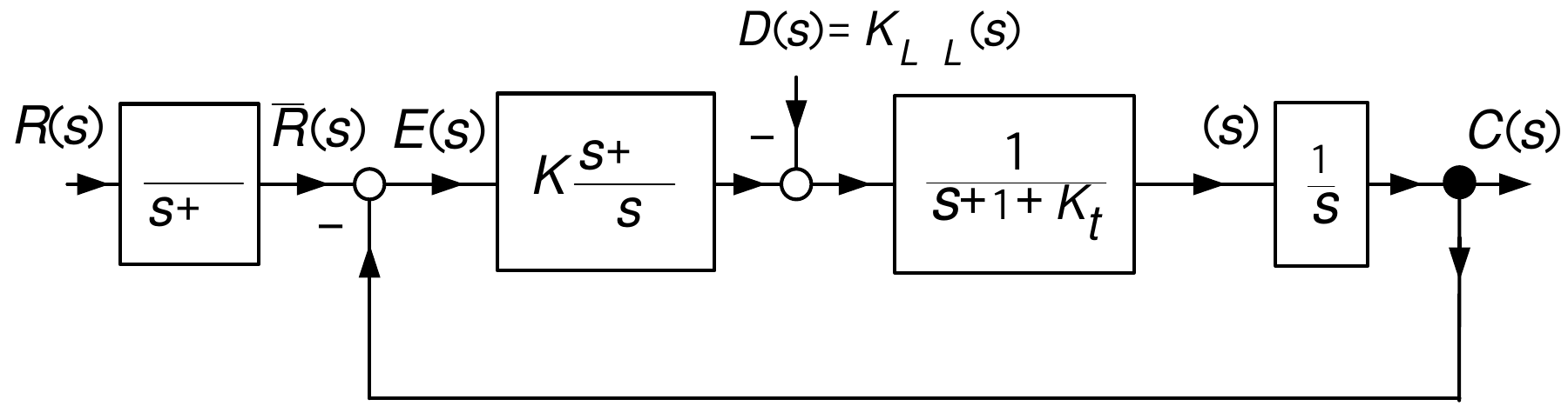
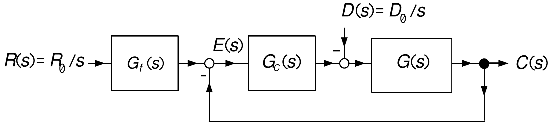
2 DOF controller:

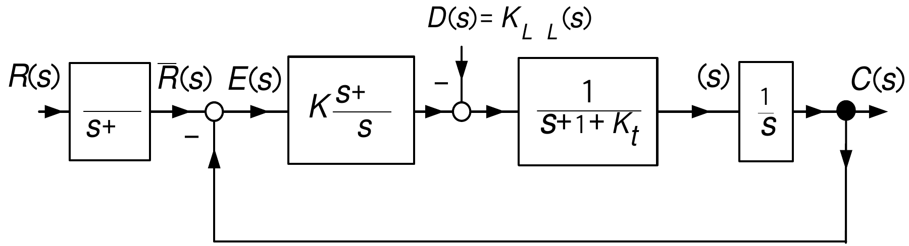
\(\dfrac{\alpha}{s+\alpha}\) is the reference input filter.

\[ C_{R}(s)=\frac{K\dfrac{s+\alpha}{s}\dfrac{1}{s+1+K_{t}}\dfrac{1}{s}} {1+K\dfrac{s+\alpha}{s}\dfrac{1}{s+1+K_{t}}\dfrac{1}{s}}\frac{\alpha} {s+\alpha}\frac{R_{0}}{s}=\frac{K(s+\alpha)}{s^{3}+(1+K_{t})s^{2}+Ks+\alpha K}\frac{\alpha}{s+\alpha}\frac{R_{0}}{s}. \]

Stable Systems with Real Poles and No Zeros Do Not Have Overshoot

\(c_{R}(\infty)=\lim_{s\rightarrow0}sC_{R}(s)=\lim_{s\rightarrow 0}\underset{\rightarrow1}{\underbrace{\dfrac{K(s+\alpha)}{s^{3}+(1+K_{t} )s^{2}+Ks+\alpha K}}}\underset{\rightarrow1}{\underbrace{\dfrac{\alpha }{s+\alpha}}}R_{0}=R_{0}.\)

Right Half-Plane Zeros

Example Right Half-Plane Zero

\(R(s)=\dfrac{R_{0}}{s},G(s)=-\dfrac{s-1}{s(s+2)}\) and \(G_{c} (s)=\dfrac{b_{1}s+b_{0}}{s+a_{0}}.\)

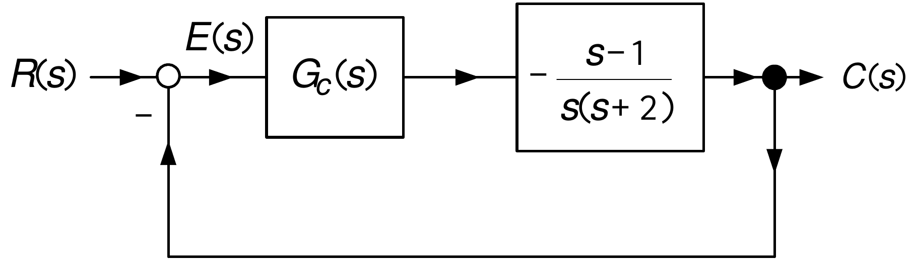
\[ \begin{aligned} E(s)=\frac{1}{1+G(s)G_{c}(s)}R(s) & =\frac{1}{1-\dfrac{s-1}{s(s+2)} \dfrac{b_{1}s+b_{0}}{s+a_{0}}}\frac{R_{0}}{s}\\ & =\frac{s(s+2)(s+a_{0})}{s(s+2)(s+a_{0})-(s-1)(b_{1}s+b_{0})}\frac{R_{0}} {s}\\ & =\frac{s(s+2)(s+a_{0})}{s^{3}+(a_{0}-b_{1}+2)s^{2}+(2a_{0}-b_{0} +b_{1})s+b_{0}}\frac{R_{0}}{s}\\ & =\frac{(s+2)(s+a_{0})}{s^{3}+(a_{0}-b_{1}+2)s^{2}+(2a_{0}-b_{0} +b_{1})s+b_{0}}R_{0}. \end{aligned} \]

Example

Right Half-Plane Zero (continued)

\(R(s)=\dfrac{R_{0}}{s},G_{c}(s)=\dfrac{b_{1}s+b_{0}}{s+a_{0}}.\)

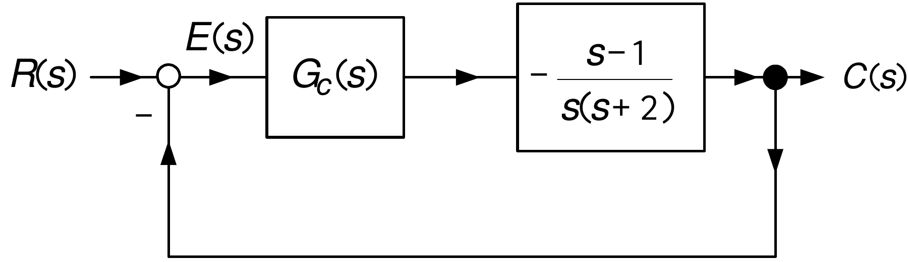
\(E(s)=\dfrac{(s+2)(s+a_{0})}{s^{3}+(a_{0}-b_{1}+2)s^{2}+(2a_{0}-b_{0} +b_{1})s+b_{0}}R_{0}.\)

Let the desired closed-loop poles be at \(-r_{1},-r_{2},-r_{3}.\)

\[ \begin{aligned} & \!\!\!\!\!\!\!\!\!\!\!\!\!\!\!\!\!\!\!\!\!\!\!\!\!\!\!\!\!\!\!\!\!\!\!\!\!\!\!\!\!\!\!\!\!\!s^{3} +(a_{0}-b_{1}+2)s^{2}+(2a_{0}-b_{0}+b_{1})s+b_{0}\\ & =(s+r_{1})(s+r_{2})(s+r_{3})\\ & =s^{3}+(r_{1}+r_{2}+r_{3})s^{2}+(r_{1}r_{2}+r_{1}r_{3}+r_{2}r_{3} )s+r_{1}r_{2}r_{3}. \end{aligned} \]

Solve:

\[ \begin{aligned} a_{0}-b_{1}+2 & =r_{1}+r_{2}+r_{3}\\ 2a_{0}+b_{1}-b_{0} & =r_{1}r_{2}+r_{1}r_{3}+r_{2}r_{3}\\ b_{0} & =r_{1}r_{2}r_{3} \end{aligned} \]

Example

Right Half-Plane Zero (continued)

\[ \begin{aligned} b_{1} & =\frac{-2(r_{1}+r_{2}+r_{3})+r_{1}r_{2}+r_{1}r_{3}+r_{2}r_{3} +r_{1}r_{2}r_{3}+4}{3}\\ a_{0} & =\frac{r_{1}+r_{2}+r_{3}+r_{1}r_{2}+r_{1}r_{3}+r_{2}r_{3}+r_{1} r_{2}r_{3}-2}{3}\\ b_{0} & =r_{1}r_{2}r_{3}. \end{aligned} \]

\[ C(s)=\frac{G(s)G_{c}(s)}{1+G(s)G_{c}(s)}R(s)=\frac{-\dfrac{s-1}{s(s+2)} \dfrac{b_{1}s+b_{0}}{s+a_{0}}}{1-\dfrac{s-1}{s(s+2)}\dfrac{b_{1}s+b_{0} }{s+a_{0}}}\frac{R_{0}}{s}=\frac{-(s-1)b_{1}(s+b_{0}/b_{1})}{(s+r_{1} )(s+r_{2})(s+r_{3})}\frac{R_{0}}{s}. \]

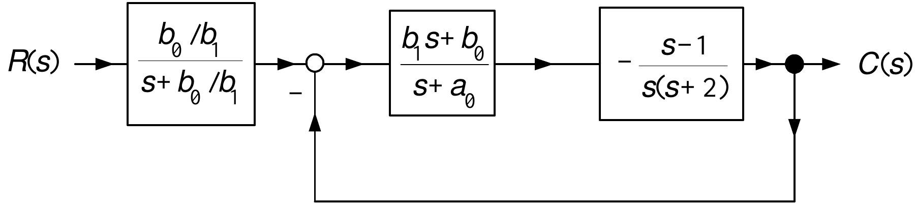
Suppose the zero at \(-b_{0}/b_{1}\) is in the open LHP so that \(\dfrac{b_{0}/b_{1}}{s+b_{0}/b_{1}}\) is a stable filter.

Put \(R(s)\) through this filter as shown.

Example

Right Half-Plane Zero (continued)

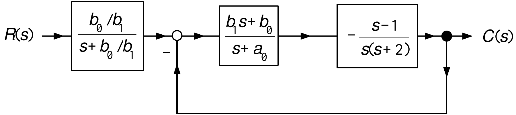
\[ \begin{aligned} \!\!\!\!\!C(s) & =\!\!\!\!\frac{-\dfrac{s-1}{s(s+2)}\dfrac{b_{1}s+b_{0} }{s+a_{0}}}{1-\dfrac{s-1}{s(s+2)}\dfrac{b_{1}s+b_{0}}{s+a_{0}}}\frac {b_{0}/b_{1}}{s+b_{0}/b_{1}}R(s)\\ & \\ & =\!\!\!\!\frac{-(s-1)b_{1}(s+b_{0}/b_{1})}{s^{3}+(a_{0}-b_{1}+2)s^{2} +(2a_{0}+b_{1}-b_{0})s+b_{0}}\frac{b_{0}/b_{1}}{s+b_{0}/b_{1}}\frac{R_{0}} {s}\\ & \\ & =\!\!\!\!\underset{G_{CL}(s)}{\underbrace{-\frac{(s-1)b_{0}}{(s+r_{1} )(s+r_{2})(s+r_{3})}}\frac{R_{0}}{s}}. \end{aligned} \]

\(G_{CL}(s)\) is stable with all real poles and only one right half-plane zero.
A theorem guarantees the step response will not have overshoot.
However, recall that the system will have undershoot.

Example

Two Right Half-Plane Zeros

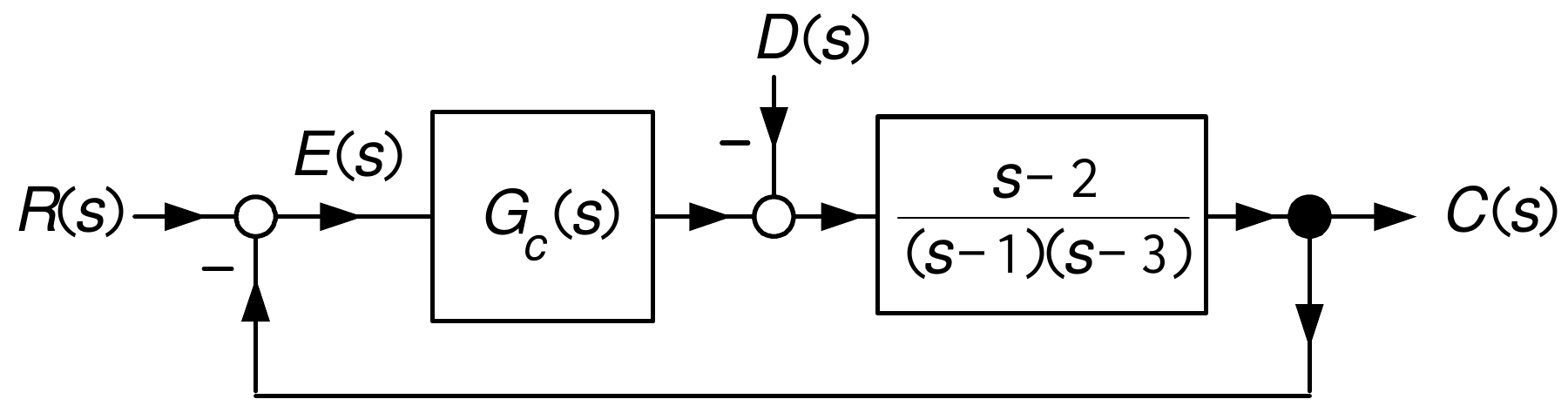
With \(\dfrac{b_{2}s^{2}+b_{1}s+b_{0}}{s+a_{0}}\dfrac{1}{s}\) we previously showed that

\[ \begin{aligned} C(s) & =\frac{G_{c}(s)G(s)}{1+G_{c}(s)G(s)}R(s)\\ & =\frac{(b_{2}s^{2}+b_{1}s+b_{0})(s-2)}{s^{4}+(a_{0}+b_{2}-4)s^{3} +(b_{1}-4a_{0}-2b_{2}+3)s^{2}+(3a_{0}+b_{0}-2b_{1})s-2b_{0}}\frac{R_{0}}{s}\\ & =\frac{(b_{2}s^{2}+b_{1}s+b_{0})(s-2)}{s^{4}+f_{3}s^{3}+f_{2}s^{2} +f_{1}s+f_{0}}\frac{R_{0}}{s}. \end{aligned} \]

where

\[ \left[ \begin{array}{c} b_{2}\\ b_{1}\\ b_{0}\\ a_{0} \end{array} \right] =\left[ \begin{array}{l} f_{0}/2+f_{1}+2f_{2}+5f_{3}+14\\ -f_{0}-2f_{1}-3f_{2}-6f_{3}-15\\ -f_{0}/2\\ -f_{0}/2-f_{1}-2f_{2}-4f_{3}-10 \end{array} \right] . \]

Example

Two Right Half-Plane Zeros (continued)

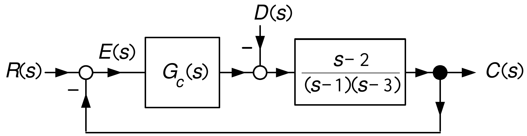
\[ C(s)=\frac{(b_{2}s^{2}+b_{1}s+b_{0})(s-2)}{s^{4}+f_{3}s^{3}+f_{2}s^{2} +f_{1}s+f_{0}}\frac{R_{0}}{s}=\frac{(b_{2}s^{2}+b_{1}s+b_{0})(s-2)}{(s+r)^{4} }\frac{R_{0}}{s} \]

where

\[ \begin{aligned} f_{3} & =r_{1}+r_{2}+r_{3}+r_{4}\\ f_{2} & =r_{1}r_{2}+r_{1}r_{3}+r_{1}r_{4}+r_{2}r_{3}+r_{2}r_{4}+r_{3}r_{4}\\ f_{1} & =r_{1}r_{2}r_{3}+r_{1}r_{2}r_{4}+r_{1}r_{3}r_{4}+r_{2}r_{3}r_{4}\\ f_{0} & =r_{1}r_{2}r_{3}r_{4} \end{aligned} \]

and \(r_{1}=r_{2}=r_{3}=r_{4}=r.\)

Example

Two Right Half-Plane Zeros (continued)

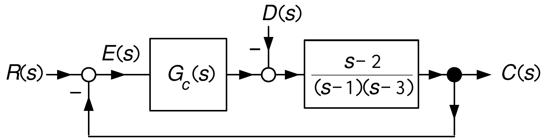
\[ C(s)=\frac{(b_{2}s^{2}+b_{1}s+b_{0})(s-2)}{(s+r)^{4}}\frac{R_{0}}{s}. \]

With \(r=1\) it turns out that

\[ b_{2}=50.5,\quad{}b_{1}=-66,\quad{}b_{0}=-0.5. \]

The zeros of the controller are the solutions to

\[ b_{2}s^{2}+b_{1}s+b_{0}=50.5s^{2}-66s-0.5=0 \]

\[ 1.3145,\quad{}-0.0075. \]

\[ C(s)=\frac{50.5(s-1.3145)(s+0.0075)(s-2)}{(s+1)^{4}}\frac{R_{0}}{s}. \]

Example

Two Right Half-Plane Zeros (continued)

\[ C(s)=\frac{50.5(s-1.3145)(s+0.0075)(s-2)}{(s+1)^{4}}\frac{R_{0}}{s}. \]

Reference filter for the two RHP zeros:

Two right half-plane zeros at \(z_{1}=2\) and \(z_{2}=1.3145.\) Form the polynomial

\[ \begin{aligned} (s-z_{1})(s-z_{2}) & =(s-1.3145)(s-2)=s^{2}-3.3145s+\underset{\omega_{0} ^{2}}{\underbrace{2.629}}\\ & \Longrightarrow G_{fz_{1}z_{2}}=\left( \frac{\omega_{0}}{s+\omega_{0} }\right) ^{2}\!\text{ where }\omega_{0}^{2}=2.629. \end{aligned} \]

Reference filter for the one LHP zero:

One left half-plane zero at \(z_{3}=-0.0075.\) Set \(\alpha=-z_{3}=0.0075.\)

\[ G_{fz_{3}}=\frac{\alpha}{s+\alpha}=\frac{0.0075}{s+0.0075}. \]

Example

Two Right Half-Plane Zeros (continued)

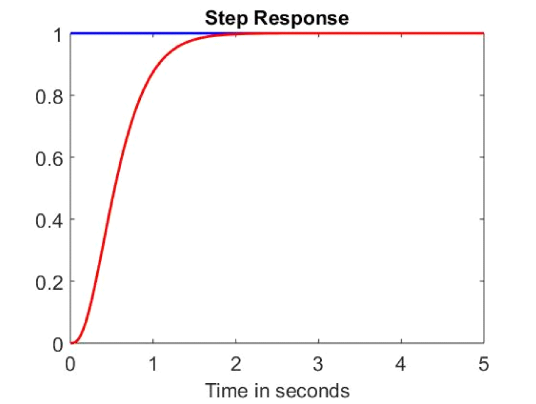
Step response with closed-loop poles set at \(-1\) and using an input reference filter.

Example

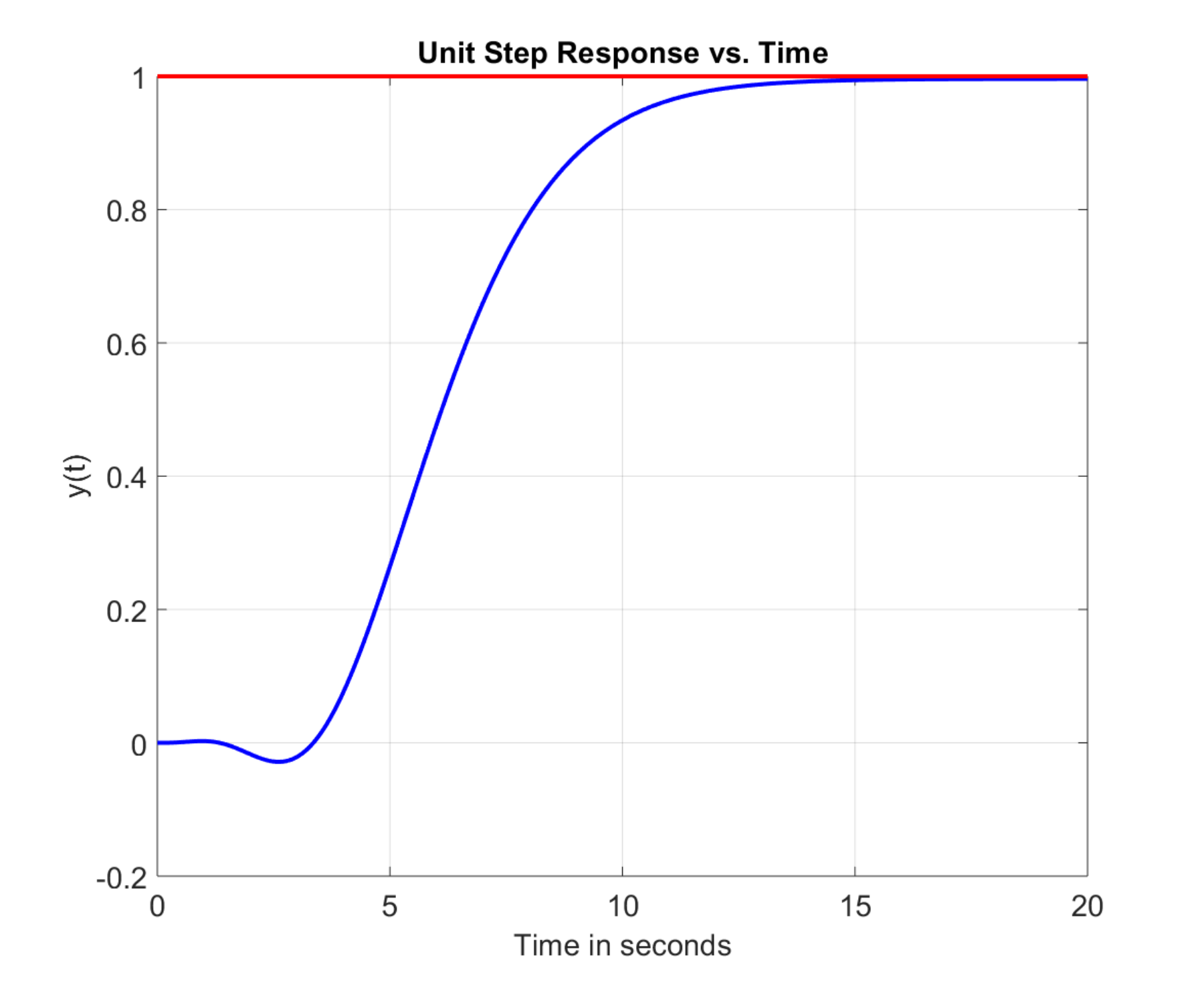
Two Right Half-Plane Zeros (continued)

The transfer function \(G(s)=\dfrac{s-2}{(s-1)(s-3)}\) is a toy example!
The poles and zeros of a physical system are never known exactly.
If the TF was really \(G(s)=\dfrac{s-2}{(s-0.9)(s-3)}\) then, using the above controller,

the closed-loop system would be unstable!
If small changes in the model result in the CL system being unstable,

we say it is not robust.
When a system has poles in the open right half-plane,

it may not be possible to find a robust controller!
Nyquist theory provides the insight into this problem.

Eliminating Overshoot with a 2 DOF Controller

Let \(G_{c}(s)G(s)\) be at least type 1 and

\[ G_{CL}(s)=\frac{G_{c}(s)G(s)}{1+G_{c}(s)G(s)}=\frac{n(s)}{d(s)}\quad{}\text{stable with real poles} \]

(a) No right half-plane zeros

\(n(s)\) has all of its roots in the open left half-plane.

\[ G_{f}(s)\triangleq\frac{n(0)}{n(s)}. \]

Then the inverse Laplace transform of

\[ C(s)=G_{f}(s)G_{CL}(s)\frac{R_{0}}{s} \]

will not have overshoot and \(c(\infty)=R_{0}\).

Eliminating Overshoot with a 2 DOF Controller

Let \(G_{c}(s)G(s)\) be at least type 1 and

\[ G_{CL}(s)=\frac{G_{c}(s)G(s)}{1+G_{c}(s)G(s)}=\frac{n(s)}{d(s)}\quad{}\text{stable with real poles} \]

(b) One right half-plane zero

\(n(s)=\bar{n}(s)(s-z).\)
\(\bar{n}(s)\) has all its roots in the open left half-plane.
\(z>0\).

\[ G_{f}(s)\triangleq\frac{\bar{n}(0)}{\bar{n}(s)}. \]

Then the inverse Laplace transform of

\[ C(s)=G_{f}(s)G_{CL}(s)\frac{R_{0}}{s} \]

will not have overshoot and \(c(\infty)=R_{0}\) (It will have undershoot).

Eliminating Overshoot with a 2 DOF Controller

Let \(G_{c}(s)G(s)\) be at least type 1 and

\[ G_{CL}(s)=\frac{G_{c}(s)G(s)}{1+G_{c}(s)G(s)}=\frac{n(s)}{d(s)}\quad{}\text{stable with real poles} \]

(c) Two right half-plane zeros

\(n(s)=\bar{n}(s)(s-z_{1})(s-z_{2})=\bar{n}(s)(s^{2}-(z_{1}+z_{2} )s+z_{1}z_{2}).\)
\(\bar{n}(s)\) has all of its roots in the open left half-plane.
\(\operatorname{Re}\{z_{1}\}>0,\operatorname{Re}\{z_{2}\}>0\) and \(\omega_{0}\triangleq\sqrt{z_{1}z_{2}}.\)

\[ G_{f}(s)\triangleq\frac{\bar{n}(0)}{\bar{n}(s)}\left( \frac{\omega_{0} }{s+\omega_{0}}\right) ^{2}. \]

Then the inverse Laplace transform of

\[ C(s)=G_{f}(s)G_{CL}(s)\frac{R_{0}}{s} \]

will not have overshoot and \(c(\infty)=R_{0}\).

Definition

Internal Stability

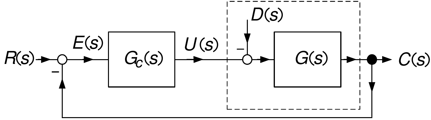
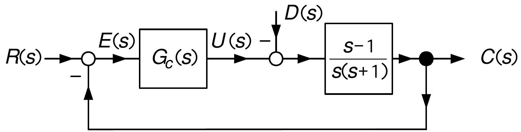
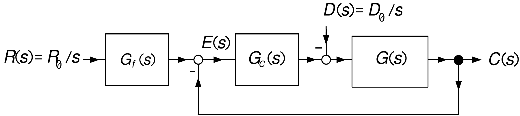
Two external inputs: \(R(s)\) and \(D(s)\).

We are interested in the responses \(E(s),U(s),C(s).\)

\[ \begin{aligned} E(s) & =\frac{1}{1+G_{c}(s)G(s)}R(s)+\frac{G(s)}{1+G_{c}(s)G(s)}D(s)\\ C(s) & =\frac{G_{c}(s)G(s)}{1+G_{c}(s)G(s)}R(s)-\frac{G(s)}{1+G_{c} (s)G(s)}D(s)\\ U(s) & =\frac{G_{c}(s)}{1+G_{c}(s)G(s)}R(s)+\frac{G_{c}(s)G(s)} {1+G_{c}(s)G(s)}D(s). \end{aligned} \]

Internal Stability

The system is said to be internally stable if these six transfer functions are stable.

Closed-Loop Characteristic Polynomial

\(G(s)=\dfrac{b(s)}{a(s)}\) is strictly proper\(,\) \(G_{c}(s)=\dfrac{b_{c} (s)}{a_{c}(s)}\) is proper.

\[ \begin{aligned} E(s) & =\frac{a_{c}(s)a(s)}{a_{c}(s)a(s)+b_{c}(s)b(s)}R(s)+\frac {a_{c}(s)b(s)}{a_{c}(s)a(s)+b_{c}(s)b(s)}D(s)\\ & \\ C(s) & =\frac{b_{c}(s)b(s)}{a_{c}(s)a(s)+b_{c}(s)b(s)}R(s)-\frac {a_{c}(s)b(s)}{a_{c}(s)a(s)+b_{c}(s)b(s)}D(s)\\ & \\ U(s) & =\frac{a(s)b_{c}(s)}{a_{c}(s)a(s)+b_{c}(s)b(s)}R(s)+\frac {b_{c}(s)b(s)}{a_{c}(s)a(s)+b_{c}(s)b(s)}D(s). \end{aligned} \]

The closed-loop characteristic polynomial is \(a_{CL}(s)\triangleq a_{c}(s)a(s)+b_{c}(s)b(s)\).
The six transfer functions are stable iff \(a_{CL}(s)\neq0\) for \(\operatorname{Re}\{s\}\geq0.\)

Polynomials

Definition Coprime Polynomials

\(a(s),b(s)\) are coprime if there is no \(s_{0}\) such that \(a(s_{0} )=b(s_{0})=0.\)

Example \(a(s)=(s+1)(s-1)\) and \(b(s)=s-1\)

Not coprime as \(a(1)=b(1)=0.\)

They both have the factor \(s-1.\)

Example \(a(s)=(s+1)(s^{2}+1)\) and\(\ b(s)=s-1.\)

\(a(s)\) and \(b(s)\) are coprime as \(b(s)=0\) only if \(s=1\) and \(a(1)\neq 0.\)

\(a(s)\) and \(b(s)\) do not have a factor in common.

\(a(s)\) and \(b(s)\) are coprime if and only if they do not have a common factor.

Definition

Coprime Transfer Functions

A transfer function \(G(s)=\dfrac{b(s)}{a(s)}\) is coprime if \(a(s)\) and \(b(s)\) are coprime.

We will always assume \(G(s)\) and \(G_{c}(s)\) are each coprime transfer functions.

Remark Suppose the transfer function of a physical system is

\[ G(s)=\frac{s+3}{s(s+1)(s+2)}. \]

There is no sense in writing this as

\[ G(s)=\frac{(s+3)(s+4)}{s(s+1)(s+2)(s+4)} \]

Similarly for \(G_{c}(s)\).

Unstable Pole-Zero Cancellation

All six transfer functions of the control system are stable if

\[ a_{c}(s)a(s)+b_{c}(s)b(s)\neq0\qquad{}\text{for}\qquad{}\operatorname{Re}\{s\}\geq0. \]

However, this can be tricky!
Don’t just look at the denominator of one of the six transfer functions.
The problem is pole-zero cancellation between \(G(s)\) and \(G_{c}(s).\)

Example

Unstable Pole-Zero Cancellation

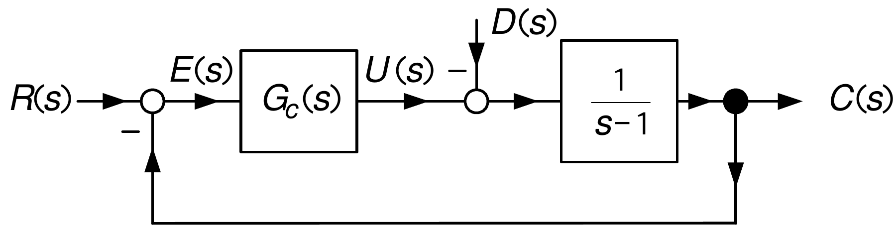
\(E(s)=\dfrac{1}{1+G_{c}(s)G(s)}R(s)+\dfrac{G(s)}{1+G_{c}(s)G(s)}D(s).\)

Let \(G_{c}(s)=\dfrac{b_{c}(s)}{a_{c}(s)}=\dfrac{s-1}{s(s+1)}.\)

\[ \begin{aligned} E_{R}(s) & =\frac{1}{1+\dfrac{s-1}{s(s+1)}\dfrac{1}{s-1}}R(s)\\ & \\ & =\frac{s(s+1)(s-1)}{s(s+1)(s-1)+(s-1)}R(s)\\ & \\ & =\frac{s(s+1)(s-1)}{(s^{2}+s+1)(s-1)}R(s)\\ & \\ & =\frac{s(s+1)}{s^{2}+s+1}R(s). \end{aligned} \]

Example

Unstable Pole-Zero Cancellation (continued)

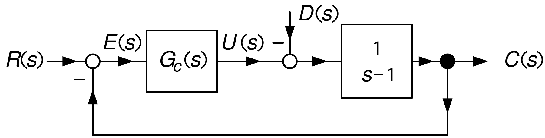
\(G_{c}(s)=\dfrac{s-1}{s(s+1)},G(s)=\dfrac{1}{s-1}\) and

\[ a_{c}(s)a(s)+b_{c}(s)b(s)=s(s+1)(s-1)+(s-1)=(s^{2}+s+1)(s-1) \]

From the previous slide:

\[ E_{R}(s)=\frac{1}{1+\underset{G_{c}(s)}{\underbrace{\dfrac{s-1}{s(s+1)}} }\underset{G(s)}{\underbrace{\dfrac{1}{s-1}}}}R(s)=\frac{s(s+1)(s-1)} {(s^{2}+s+1)(s-1)}\frac{R_{0}}{s}=\frac{s+1}{s^{2}+s+1}R_{0} \]

The transfer function \(\dfrac{E_{R}(s)}{R(s)}=\dfrac{s(s+1)}{s^{2}+s+1}\) is stable after the cancellation.
Note this was an unstable pole-zero cancellation.
Such unstable pole-zero cancellations will not work in physical systems.

Example

Unstable Pole-Zero Cancellation (continued)

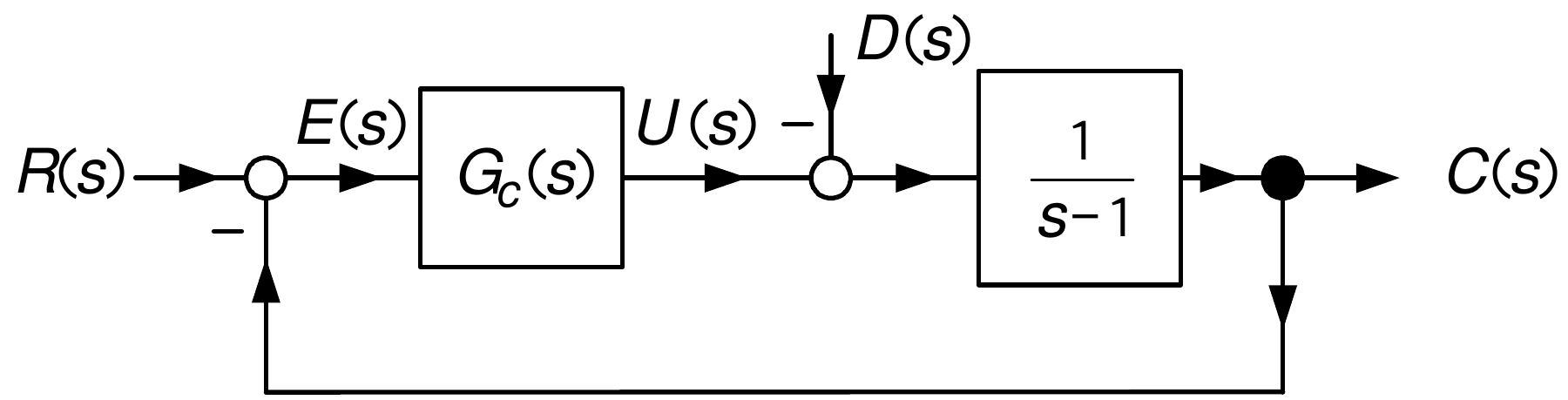
\[ \!\!\!\!\!E_{D}(s)=\frac{\dfrac{1}{s-1}}{1+\dfrac{s-1}{s(s+1)}\dfrac{1}{s-1} }D(s)=\frac{s(s+1)}{s(s+1)(s-1)+(s-1)}\frac{D_{0}}{s}=\frac{s(s+1)} {(s^{2}+s+1)(s-1)}\frac{D_{0}}{s}. \]

The TF \(\dfrac{E_{D}(s)}{D(s)}=\dfrac{s(s+1)}{(s^{2}+s+1)(s-1)}\) is unstable due to the pole at \(s=1.\)
This results in \(|e_{D}(t)|\rightarrow\infty.\)
This system is not internally stable.
\(\dfrac{E_{R}(s)}{R(s)}\) is stable (due to unstable pole-zero cancellation), but \(\dfrac{E_{D}(s)}{D(s)}\) is not stable.

Example

Unstable Pole-Zero Cancellation

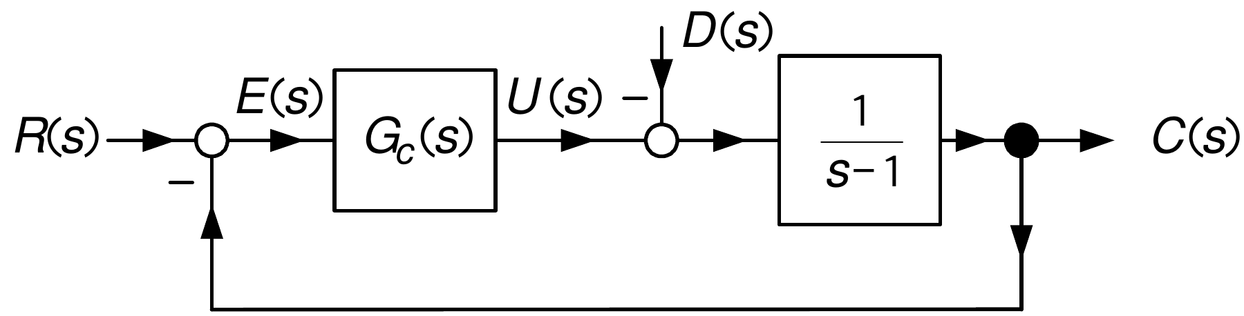
Let \(G_{c}(s)=\dfrac{s-1}{s(s+1)}\). Even with \(D(s)=0\) this controller will not work.

Any model is an approximation of the physical system.

Though we write \(G(s)\triangleq\dfrac{1}{s-1}\) it is really \(G(s)\triangleq \dfrac{1}{s-p}\) where \(p\approx1.\)

\[ E_{R}(s)=\frac{1}{1+\dfrac{s-1}{s(s+1)}\dfrac{1}{s-p}}R(s)=\frac{s(s+1)\left( s-p\right) }{s^{3}+(1-p)s^{2}+(1-p)s-1}\frac{R_{0}}{s}. \]

For \(p\neq1\) there is no cancellation!
\(s^{3}+(1-p)s^{2}+(1-p)s-1\) is unstable for all \(p\)!
\(\left. s^{3}+(1-p)s^{2}+(1-p)s-1\right\vert _{p=1}=(s^{2} +s+1)(s-1)\)

\(\qquad\blacktriangleright\) Only if \(p\) is exactly \(1\) is there cancellation. This won’t happen!

Example

Unstable Pole-Zero Cancellation

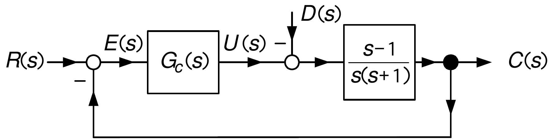
\(G_{c}(s)=\dfrac{K}{s-1}\) and suppose we have (unrealistic) exact cancellation.

\[ \begin{aligned} E(s) & =\frac{1}{1+\dfrac{K}{s-1}\dfrac{s-1}{s(s+1)}}R(s)+\frac{\dfrac {s-1}{s(s+1)}}{1+\dfrac{K}{s-1}\dfrac{s-1}{s(s+1)}}D(s)\\ & \\ & =\frac{s(s+1)(s-1)}{(s^{2}+s+K)(s-1)}\frac{R_{0}}{s}+\frac{(s-1)^{2}} {(s^{2}+s+K)(s-1)}\frac{D_{0}}{s}\\ & \\ & =\frac{s+1}{s^{2}+s+K}R_{0}+\frac{s-1}{s^{2}+s+K}\frac{D_{0}}{s}. \end{aligned} \]

With this ” perfect” unstable pole-zero cancellation and \(K>0,\) \(sE(s)\) is stable.

\(\Longrightarrow\) \(e(\infty)=-\dfrac{D_{0}}{K}.\) Won’t work! (See next slide.)

Example

Unstable Pole-Zero Cancellation (continued)

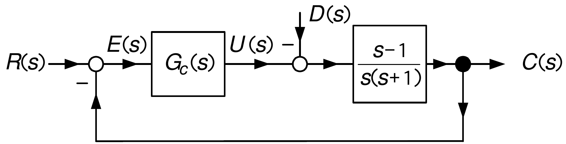
\(G_{c}(s)=\dfrac{K}{s-1}.\)

\[ \begin{aligned} U(s) & =\frac{G_{c}(s)}{1+G_{c}(s)G(s)}R(s)+\frac{G_{c}(s)G(s)} {1+G_{c}(s)G(s)}D(s)\\ & =\frac{\dfrac{K}{s-1}}{1+\dfrac{K}{s-1}\dfrac{s-1}{s(s+1)}}R(s)+\frac {\dfrac{K}{s-1}\dfrac{s-1}{s(s+1)}}{1+\dfrac{K}{s-1}\dfrac{s-1}{s(s+1)}}D(s)\\ & =\frac{s(s+1)K}{(s^{2}+s+K)(s-1)}\frac{R_{0}}{s}+\frac{K}{s^{2}+s+K} \frac{D_{0}}{s}. \end{aligned} \]

\(R(s)=R_{0}/s\) will cause the input \(u(t)\) to the physical system to be unbounded.
Even with perfect (impossible) pole-zero cancellation, \(G_{c} (s)=\dfrac{K}{s-1}\) is not viable.

Example

Unstable Pole-Zero Cancellation

More Realistic View

In reality \(G(s)=\dfrac{b(s)}{a(s)}=\dfrac{s-z}{s(s+1)}\) with \(z\approx1,\) but \(z\neq1.\)

\[ E_{R}(s)=\frac{1}{1+\dfrac{1}{s-1}\dfrac{s-z}{s(s+1)}}R(s)=\frac {s(s+1)(s-1)}{s^{3}-z}R_{0} \]

Only if \(z=1\) does \(s^{3}-z\) equal \((s-1)(s^{2}+s+1)\).

Pole–Zero Cancellation Between \(G_{CL}(s)\) and \(R(s),D(s)\)

\(G_{CL}(s)\) and \(R(s),D(s)\)

Unstable pole-zero cancellation between \(G(s)\) and \(G_{c}(s)\) never works.
We do unstable pole-zero cancellations between \(G_{CL}(s)=\dfrac {G_{c}(s)G(s)}{1+G_{c}(s)G(s)}\) and \(R(s),D(s)!\)

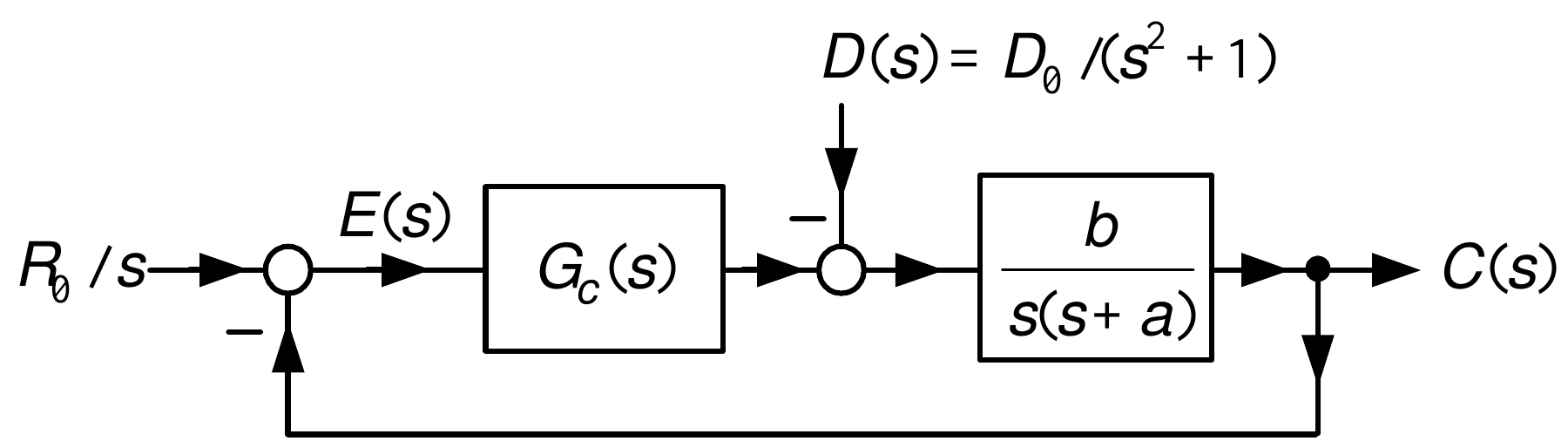
\[ \begin{aligned} \!\!\!\!\!\!\!\!\!\!\!\!\!\!E_{D}(s) & =\!\!\!\frac{G(s)}{1+G_{c} (s)G(s)}D(s)=\frac{\dfrac{b}{s(s+a)}}{1+\underset{G_{c}(s)}{\underbrace{\dfrac {b_{3}s^{3}+b_{2}s^{2}+b_{1}s+b_{0}}{s+a_{0}}\dfrac{1}{s^{2}+1}}}\dfrac {b}{s(s+a)}}\frac{D_{0}}{s^{2}+1}\\ & \\ \!\!\!\!\!\!\!\!\!\!\!\!\!\! & =\!\!\!\underset{G_{CL}(s)}{\underbrace{\frac {(s+a_{0})(s^{2}+1)b}{s^{5}+(a+a_{0})s^{4}+(aa_{0}+bb_{3}+1)s^{3} +(a+a_{0}+bb_{2})s^{2}+(aa_{0}+bb_{1})s+bb_{0}}}}\frac{D_{0}}{s^{2}+1}\\ & \\ \!\!\!\!\!\!\!\!\!\!\!\!\!\! & =\!\!\!\frac{(s+a_{0})b}{s^{5}+f_{4} s^{4}+f_{3}s^{3}+f_{2}s^{2}+f_{1}s+f_{0}}D_{0}. \end{aligned} \]

Pole–Zero Cancellation Between \(G_{CL}(s)\) and \(R(s),D(s)\)

\(G_{CL}(s)\) and \(R(s)\) & \(D(s)\)

\[ \begin{aligned} \!\!\!\!\!E_{D}(s) & =\underset{G_{CL}(s)}{\underbrace{\frac{(s+a_{0} )(s^{2}+1)b}{s^{5}+(a+a_{0})s^{4}+(aa_{0}+bb_{3}+1)s^{3}+(a+a_{0}+bb_{2} )s^{2}+(aa_{0}+bb_{1})s+bb_{0}}}}\frac{D_{0}}{s^{2}+1}\\ & \\ & =\frac{(s+a_{0})b}{s^{5}+f_{4}s^{4}+f_{3}s^{3}+f_{2}s^{2}+f_{1}s+f_{0}} D_{0}. \end{aligned} \]

Cancelled the \(1/(s^{2}+1)\) of \(D(s)\) with the \(s^{2}+1\) in the numerator of \(E_{D}(s)/D(s)=G_{CL}(s).\)

Now suppose the disturbance is really

\[ D(s)=\frac{D_{0}}{s^{2}+1+\epsilon}. \]

Then

\[ \begin{aligned} E_{D}(s) & =\frac{(s+a_{0})(s^{2}+1)b}{s^{5}+f_{4}s^{4}+f_{3}s^{3}+f_{2} s^{2}+f_{1}s+f_{0}}\frac{D_{0}}{s^{2}+1+\epsilon}\\ & =\frac{(s+a_{0})(s^{2}+1+\epsilon-\epsilon)b}{s^{5}+f_{4}s^{4}+f_{3} s^{3}+f_{2}s^{2}+f_{1}s+f_{0}}\frac{D_{0}}{s^{2}+1+\epsilon}\\ & =\frac{(s+a_{0})b}{s^{5}+f_{4}s^{4}+f_{3}s^{3}+f_{2}s^{2}+f_{1}s+f_{0}} D_{0}-\underset{H(s)}{\underbrace{\frac{(s+a_{0})b}{s^{5}+f_{4}s^{4} +f_{3}s^{3}+f_{2}s^{2}+f_{1}s+f_{0}}}}\frac{\epsilon D_{0}}{s^{2}+1+\epsilon}. \end{aligned} \]

Pole–Zero Cancellation Between \(G_{CL}(s)\) and \(R(s),D(s)\)

\(G_{CL}(s)\) and \(R(s),D(s)\)

\[ E_{D}(s)=\frac{(s+a_{0})b}{s^{5}+f_{4}s^{4}+f_{3}s^{3}+f_{2}s^{2}+f_{1} s+f_{0}}D_{0}-\underset{H(s)}{\underbrace{\frac{(s+a_{0})b}{s^{5}+f_{4} s^{4}+f_{3}s^{3}+f_{2}s^{2}+f_{1}s+f_{0}}}}\frac{\epsilon D_{0}} {s^{2}+1+\epsilon}. \]

As \(H(s)\) is stable

\[ e_{D}(t)\rightarrow-\epsilon D_{0}|H(j\sqrt{1+\epsilon})|\sin\!\left( (\sqrt{1+\epsilon})t+ \angle H(j\sqrt{1+\epsilon})\right) \!. \]

The error \(e_{D}(t)\nrightarrow0\), but does remain bounded and small (assuming \(\epsilon\) is small).
The six closed-loop system transfer functions are stable with closed-loop characteristic polynomial

\[ \begin{aligned} & \!\!\!\!\!\!\!\!\!\!\!\!\!\!\!\!\!\!\!\!s^{5}+(a+a_{0})s^{4}+(aa_{0} +bb_{3}+1)s^{3}+(a+a_{0}+bb_{2})s^{2}+(aa_{0}+bb_{1})s+bb_{0}\\ & \\ & =s^{5}+f_{4}s^{4}+f_{3}s^{3}+f_{2}s^{2}+f_{1}s+f_{0} \end{aligned} \]

Pole–Zero Cancellation Between \(G_{CL}(s)\) and \(R(s),D(s)\)

\(G_{CL}(s)\) and \(R(s),D(s)\)

No physical system can handle unbounded reference or disturbance inputs.

We take them to be bounded in applications.
Bounded disturbances \(D(s)\) have simple poles on the \(j\omega\) axis.

E.g., \(D(s)=D_{0}/s,D(s)=D_{0}/(s^{2}+\omega^{2}).\)
An inexact cancellation between \(\dfrac{E_{D}(s)}{D(s)}=\dfrac {G(s)}{1+G_{c}(s)G(s)}\) and \(D(s)\)

still results in a bounded error signal.
Bounded reference inputs also have simple poles on the \(j\omega\) axis.

E.g., \(R(s)=R_{0}/s,R(s)=R_{0}/(s^{2}+\omega^{2}).\)
An inexact cancellation between \(\dfrac{E_{R}(s)}{R(s)}=\dfrac {1}{1+G_{c}(s)G(s)}\) and \(R(s)\)

results in bounded error signal.

Remark Ramp reference inputs are unbounded, i.e., \(R(s)=\omega _{0}/s^{2}\) or \(r(t)=tu_{s}(t).\)

In any application the ramp will only be applied for a finite time. For example

\[ r(t)=\left\{ \begin{array}{ll} \omega_{0}t, & 0\leq t\leq\theta_{0}/\omega_{0},\\ \theta_{0}, & \theta_{0}/\omega_{0}<t. \end{array} \right. \]

This is a bounded reference signal.

Control of Aircraft Pitch - 2 DOF Approach

\[ \frac{\theta(s)}{\delta(s)}=G(s)=\dfrac{1.51s+0.1774}{s^{3}+0.739s^{2} +0.921s}. \]

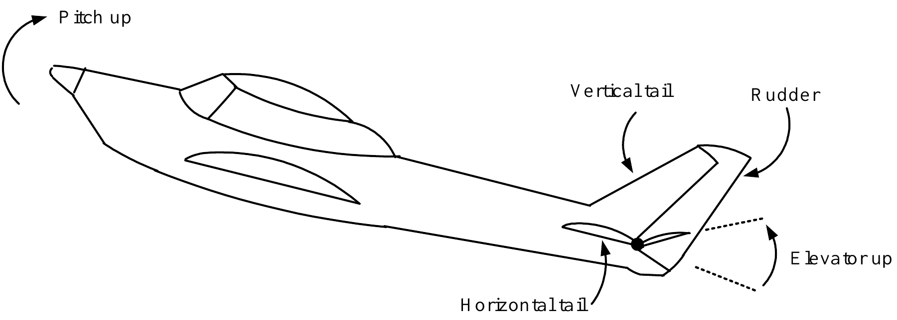
Reference Step Input: \(r(t)=0.2u_{s}(t)\) radians (\(11\) degrees) to pitch up.

Actuator Constraint: Elevator deflection is restricted to \(-25^{\circ}\leq\delta\leq25^{\circ}.\)

Design Specifications:

(1) Overshoot less than 10%.

(2) Rise time less than 2 seconds.

(3) Settling time less than 10 seconds.

(4) Steady-state error less than 2%.

Disturbances due to wind gusts are modeled as an equivalent input to the elevator.

Control of Aircraft Pitch - 2 DOF Approach

\[ \frac{\theta(s)}{\delta(s)}=G(s)=\dfrac{1.51s+0.1774}{s^{3}+0.739s^{2} +0.921s}\qquad{}\text{and}\qquad{}G_{c}(s)=\dfrac{b_{3}s^{3}+b_{2}s^{2}+b_{1}s+b_{0} }{s^{2}+a_{1}s+a_{0}}\dfrac{1}{s}. \]

\[ \begin{aligned} \frac{C(s)}{R(s)}\!\!\!\!\! & =\!\!\!\!\!\!\frac{\dfrac{b_{3}s^{3}+b_{2} s^{2}+b_{1}s+b_{0}}{s^{2}+a_{1}s+a_{0}}\dfrac{1}{s}\dfrac{1.51s+0.1774} {s^{3}+0.739s^{2}+0.921s}}{1+\dfrac{b_{3}s^{3}+b_{2}s^{2}+b_{1}s+b_{0}} {s^{2}+a_{1}s+a_{0}}\dfrac{1}{s}\dfrac{1.51s+0.1774}{s^{3}+0.739s^{2}+0.921s} }\\ & \\ \!\!\!\!\! & =\!\!\!\!\!\!\!\frac{(b_{2}s^{2}+b_{1}s+b_{0})(1.51s+0.1774)} {s(s^{2}+a_{1}s+a_{0})(s^{3}+0.739s^{2}+0.921s)+(b_{3}s^{3}+b_{2}s^{2} +b_{1}s+b_{0})(1.51s+0.1774)}\\ & \\ \!\!\!\!\! & =\!\!\!\!\!\!\frac{(b_{2}s^{2}+b_{1}s+b_{0})(1.51s+0.1774)} {a_{CL}(s)} \end{aligned} \]

Control of Aircraft Pitch - 2 DOF Approach

\[ \begin{aligned} \frac{C(s)}{R(s)} & =\frac{(b_{2}s^{2}+b_{1}s+b_{0})(1.51s+0.1774)} {a_{CL}(s)}\\ a_{CL}(s)\!\!\! & =\!\!\!s^{6}+(a_{1}+\!0.739)s^{5}+(a_{0}+\!0.739a_{1} +\!1.51b_{3}+\!0.921)s^{4}+\\ & \!\!(0.739a_{0}+\!0.921a_{1}+\!1.51b_{2}+\!0.1774b_{3})s^{3}\!+(0.921a_{0} +1.51b_{1}+0.1774b_{2})s^{2}+\\ & (1.51b_{0}+0.1774b_{1})s+0.1774b_{0}.\\ a_{CL}(s) & =s^{6}+f_{5}s^{5}+f_{4}s^{4}+f_{3}s^{3}+f_{2}s^{2}+f_{1}s+f_{0} \end{aligned} \]

\[ \left[ \begin{array}{c} f_{5}\\ f_{4}\\ f_{3}\\ f_{2}\\ f_{1}\\ f_{0} \end{array} \right] =\left[ \begin{array}{cccccc} 0 & 0 & 0 & 0 & 1 & 0\\ 1.51 & 0 & 0 & 0 & 0.739 & 1\\ 0.1774 & 1.51 & 0 & 0 & 0.921 & 0.739\\ 0 & 0.1774 & 1.51 & 0 & 0 & 0.921\\ 0 & 0 & 0.1774 & 1.51 & 0 & 0\\ 0 & 0 & 0 & 0.1774 & 0 & 0 \end{array} \right] \left[ \begin{array}{c} b_{3}\\ b_{2}\\ b_{1}\\ b_{0}\\ a_{1}\\ a_{0} \end{array} \right] +\left[ \begin{array}{c} 0.739\\ 0.921\\ 0\\ 0\\ 0\\ 0 \end{array} \right] \]

Control of Aircraft Pitch - 2 DOF Approach

How do we choose \(a_{CL}(s)=s^{6}+f_{5}s^{5}+f_{4}s^{4}+f_{3}s^{3}+f_{2} s^{2}+f_{1}s+f_{0}?\)

\[ \left[ \begin{array}{c} b_{3}\\ b_{2}\\ b_{1}\\ b_{0}\\ a_{1}\\ a_{0} \end{array} \right] \!\!=\!\!\left[ \!\! \begin{array}{cccccc} 0 & 0 & 0 & 0 & 1 & 0\\ 1.51 & 0 & 0 & 0 & 0.739 & 1\\ 0.1774 & 1.51 & 0 & 0 & 0.921 & 0.739\\ 0 & 0.1774 & 1.51 & 0 & 0 & 0.921\\ 0 & 0 & 0.1774 & 1.51 & 0 & 0\\ 0 & 0 & 0 & 0.1774 & 0 & 0 \end{array} \!\!\right] ^{-1}\!\!\left( \!\!\left[ \begin{array}{c} f_{5}\\ f_{4}\\ f_{3}\\ f_{2}\\ f_{1}\\ f_{0} \end{array} \right] \!\!-\!\!\left[ \begin{array}{c} 0.739\\ 0.921\\ 0\\ 0\\ 0\\ 0 \end{array} \right] \!\!\right) \]

Important Comments on Pole Placement

The choice of location for the closed-loop poles is crucial for good performance.
Want the closed-loop poles far in the left half-plane for a fast response.
The zeros of the controller cannot be chosen.
If possible, avoid controllers with zeros in the right half-plane (undershoot).
Zeros in the LHP can be eliminated by \(G_{f}(s).\)
Do not saturate the actuator.

Typically not any easy task to choose the location of the closed-loop poles.

Control of Aircraft Pitch - 2 DOF Approach

Put one of the closed-loop poles at \(-0.1774/1.51=-0.1175\)

to cancel the zero of \(G(s)\) at this location.
Then \(a_{CL}(s)\) has the form

\[ a_{CL}(s)=(s+0.1175)(s+r)(s^{2}+2\zeta_{1}\omega_{n1}s+\omega_{n1}^{2} )(s^{2}+2\zeta_{2}\omega_{n2}s+\omega_{n2}^{2}). \]

The ” tuning” process now consists of varying \(r,\zeta_{1},\omega_{n1},\zeta_{2},\omega_{n2}.\)
After each choice check if the zeros of \(G_{c}(s)\) are in the open LHP.
- If not, then a new set of values for \(r,\zeta_{1},\omega_{n1},\zeta _{2},\omega_{n2}\) are chosen.
With the zeros of \(G_{c}(s)\) in the open LHP check:
- If the specifications are met.
- If the actuator does not saturate.
Tried choosing all the CLP to be real and negative.
- Kept resulting in zeros of \(G_{c}(s)\) in the open right-half plane.
After quite a bit of trial and error \(a_{CL}(s)\) was chosen to be

\[ a_{CL}(s)=(s+0.1175)(s+1.6)(s^{2}+5s+25)(s^{2}+5s+25). \]

Control of Aircraft Pitch - 2 DOF Approach

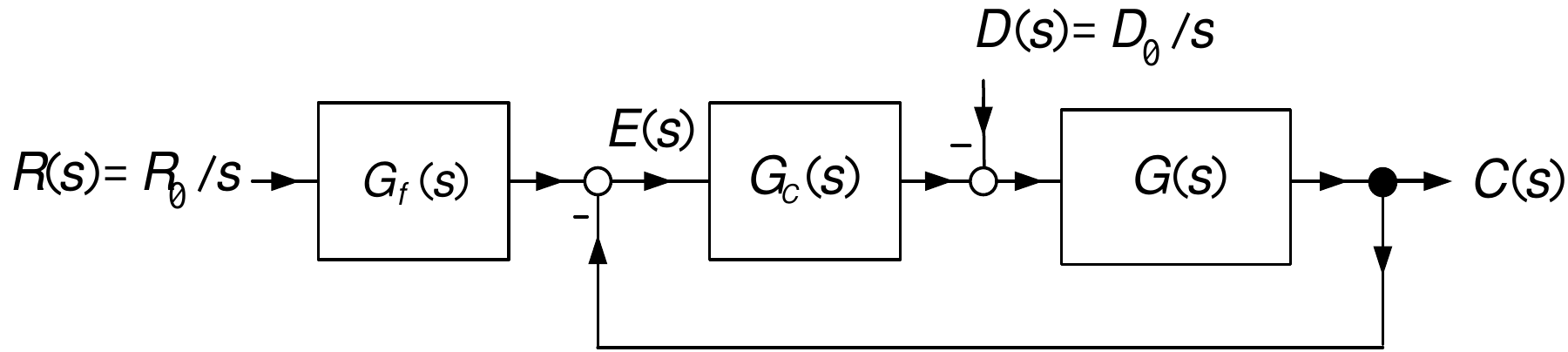
\[ \begin{aligned} G_{c}(s) & =\frac{54.34s^{3}+238.4s^{2}+678.8s+662.3}{s^{2}+10.98s+1.28} \frac{1}{s}\\ & \\ & =\frac{54.34(s+1.49)(s-[-1.45+j2.47])(s-[-1.45-j2.47])}{(s+0.1175)(s+10.86)} \frac{1}{s}. \end{aligned} \]

The zeros of \(G_{c}(s)\) are all in the open left-half plane.
\(G_{c}(s)\) has one pole at \(-0.1175\) to cancel the zero of \(G(s)\) at \(-0.1175.\)
\(G_{f}(s)\triangleq\dfrac{b_{0}}{b_{3}s^{3}+b_{2}s^{2}+b_{1}s+b_{0} }=\dfrac{662.3}{54.34s^{3}+238.4s^{2}+678.8s+662.3}\)

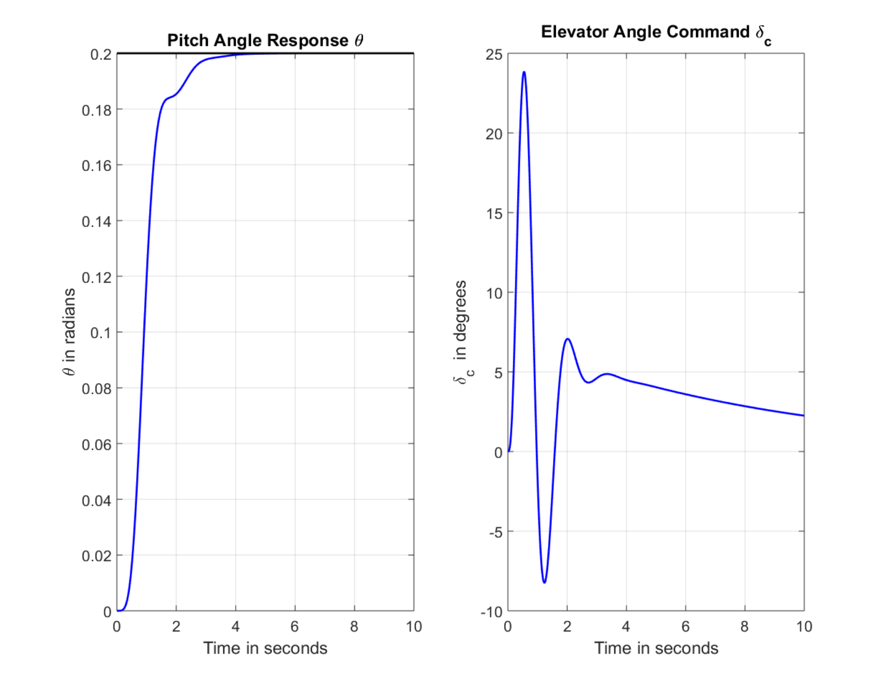
Control of Aircraft Pitch - 2 DOF Approach

The rise time is about \(1.5\) seconds.
The overshoot is zero.
The \(2\%\) settling time is \(3.1\) seconds with zero steady-state error.

Pole Placement, 2-DoF Controllers, and Internal Stability

Contents