System Responses

System Modeling and Control · Chapter 8

John N. Chiasson and Aykut C. Satici

First-Order Responses and Motor Identification
Second-Order Transient Response and Closed-Loop Poles
Peak Time, Overshoot, Settling Time, and Rise Time
Gain Selection and Motor-Parameter Identification
Effects of Zeros and Higher-Order Poles

First-Order Systems

Speed Response of a DC motor

With \(L=0,a\triangleq\dfrac{f+K_{b}K_{T}/R}{J},b\triangleq\dfrac{K_{T}}{RJ},K_{L}=\dfrac{R}{K_{T}}\):

Time Constant Form

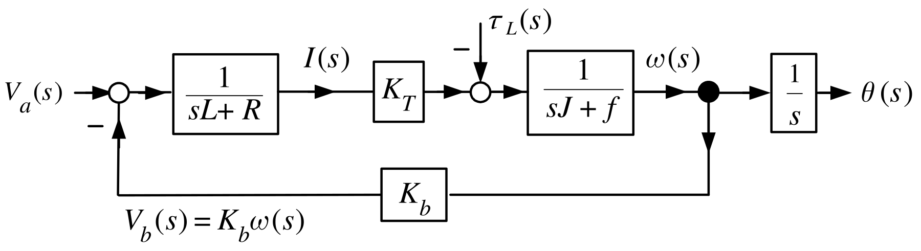
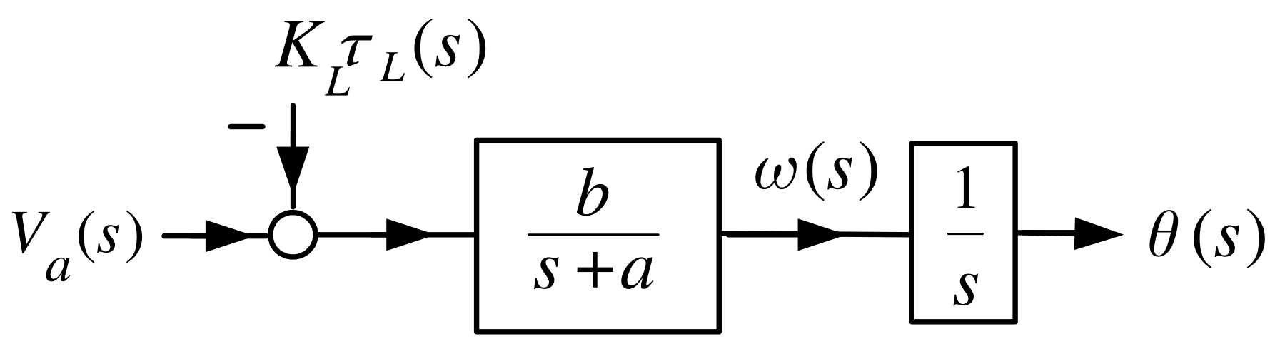
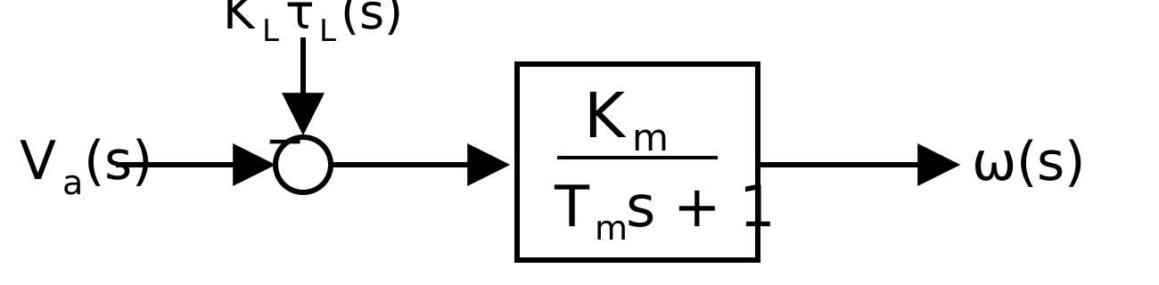
\(T_{m}\triangleq1/a,K_{m}\triangleq b/a.\)

Speed Response of a DC motor

Compute \(\omega(t)\) due to a step input voltage.
\(\omega(s)=\dfrac{K_{m}}{T_{m}s+1}V_{a}(s)-\dfrac{K_{m}}{T_{m}s+1}K_{L}\tau_{L}(s).\)
Let \(\tau_{L}=0\) and set

\[ G(s)=\frac{K_{m}}{T_{m}s+1}. \]

A common form for a first-order \(G(s).\)
- Normally the leading coefficient in \(s\) of the denominator is \(1\)!
Step input voltage \(V_{a}(s)=\dfrac{V_{0}}{s}\):

\[ \omega(s)=\frac{K_{m}}{T_{m}s+1}\frac{V_{0}}{s}=V_{0}K_{m}\!\left( \frac {1}{s}-\frac{1}{s+1/T_{m}}\right) \]

and inverse LT

\[ \omega(t)=V_{0}K_{m}(1-e^{-t/T_{m}})u_{s}(t). \]

Speed Response of a DC motor

\[ \begin{array}{c|l} \hline t & \frac{\omega(t)}{V_{0}K_{m}}=1-e^{-t/T_{m}}\\\hline 0 & 1-e^{-0}=0\\\hline T_{m} & 1-e^{-1}=0.632\\\hline 2T_{m} & 1-e^{-2}=0.86\\\hline 3T_{m} & 1-e^{-3}=0.95\\\hline 4T_{m} & 1-e^{-4}=0.98\\\hline \end{array} \]

Plot \(\omega(t)=V_{0}K_{m}(1-e^{-t/T_{m}})u_{s}(t).\)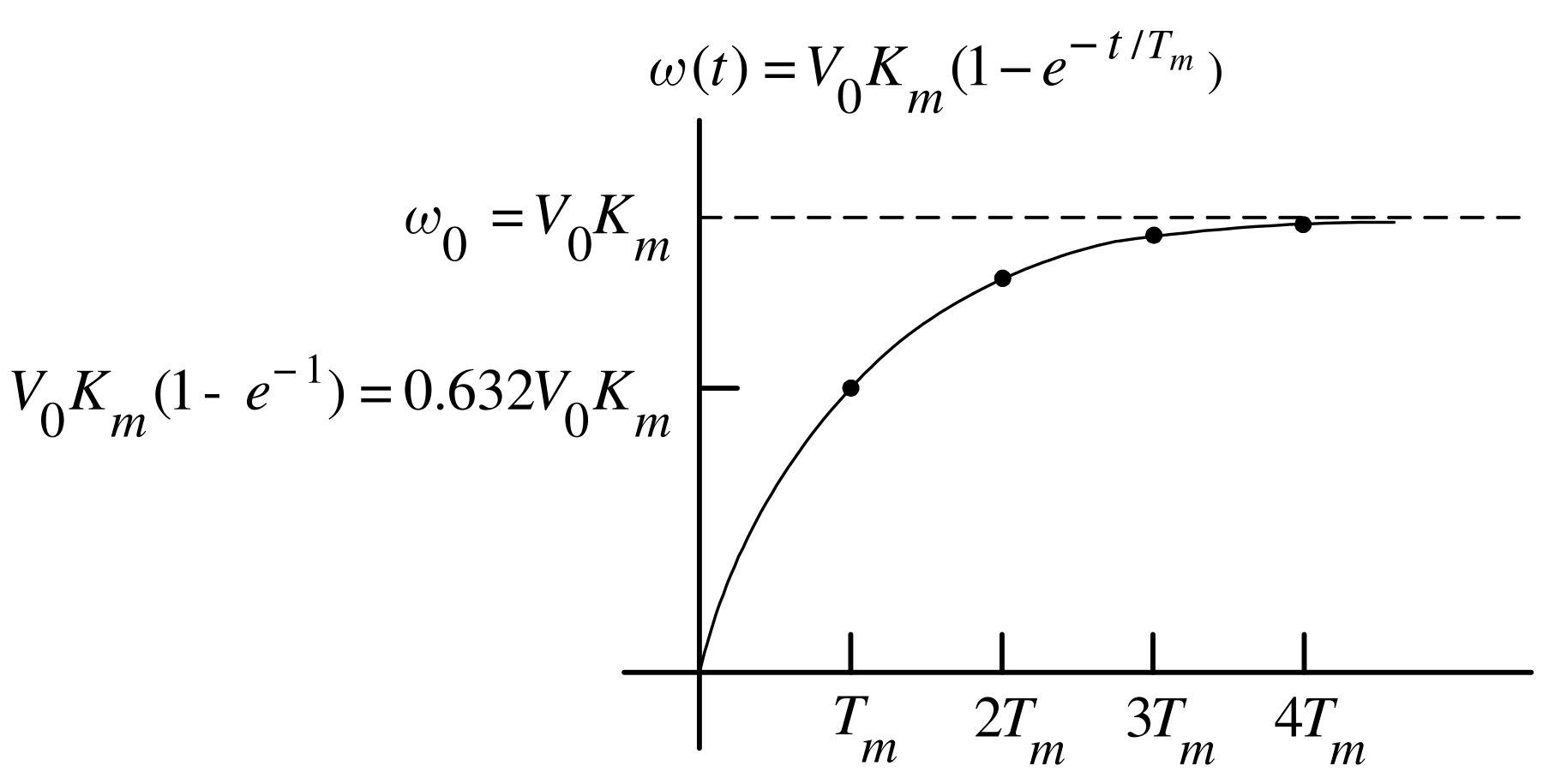

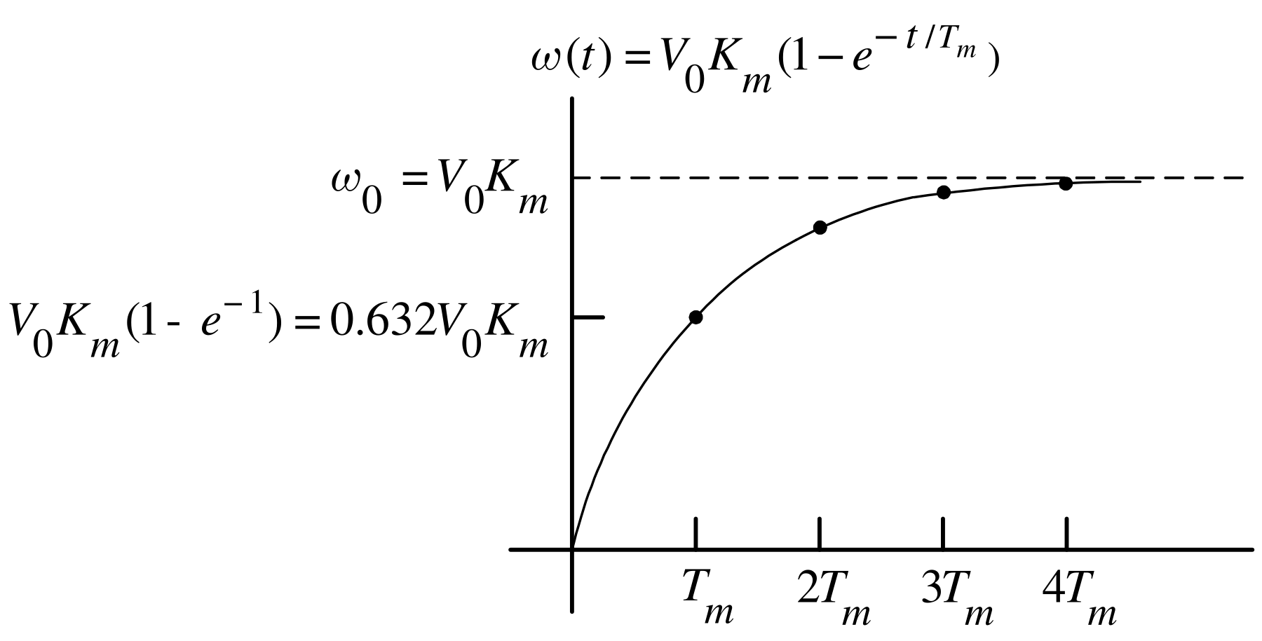
Speed Response of a DC motor

\(T_{m}\) is the time constant and its units are in seconds.
The smaller the value of \(T_{m}\) the faster the system responds.

Example Let \(\omega_{0}\) be the desired final angular speed. Set \(V_{0}=\dfrac{\omega_{0}}{K_{m}}.\)

With step input voltage of \(v_{a}(t)=\dfrac{\omega_{0}}{K_{m}}u_{s}(t)\rightarrow\omega(t)=\omega_{0}(1-e^{-t/T_{m}})u_{s}(t).\)

\(\left. \left( 1-e^{-t/T_{m}}\right) \right\vert _{t=4T_{m}}=0.98\Longrightarrow\omega(t)\) is within \(2\%\) of \(\omega_{0}\).
That is, for \(t\geq4T_{m}\) we have \(0.98\omega_{0}\leq\omega _{0}(1-e^{-t/T_{m}})\leq\omega_{0}\).
The smaller the value of \(T_{m}\), the faster \(\omega(t)\) is within \(2\%\) of its final value \(\omega_{0}.\)

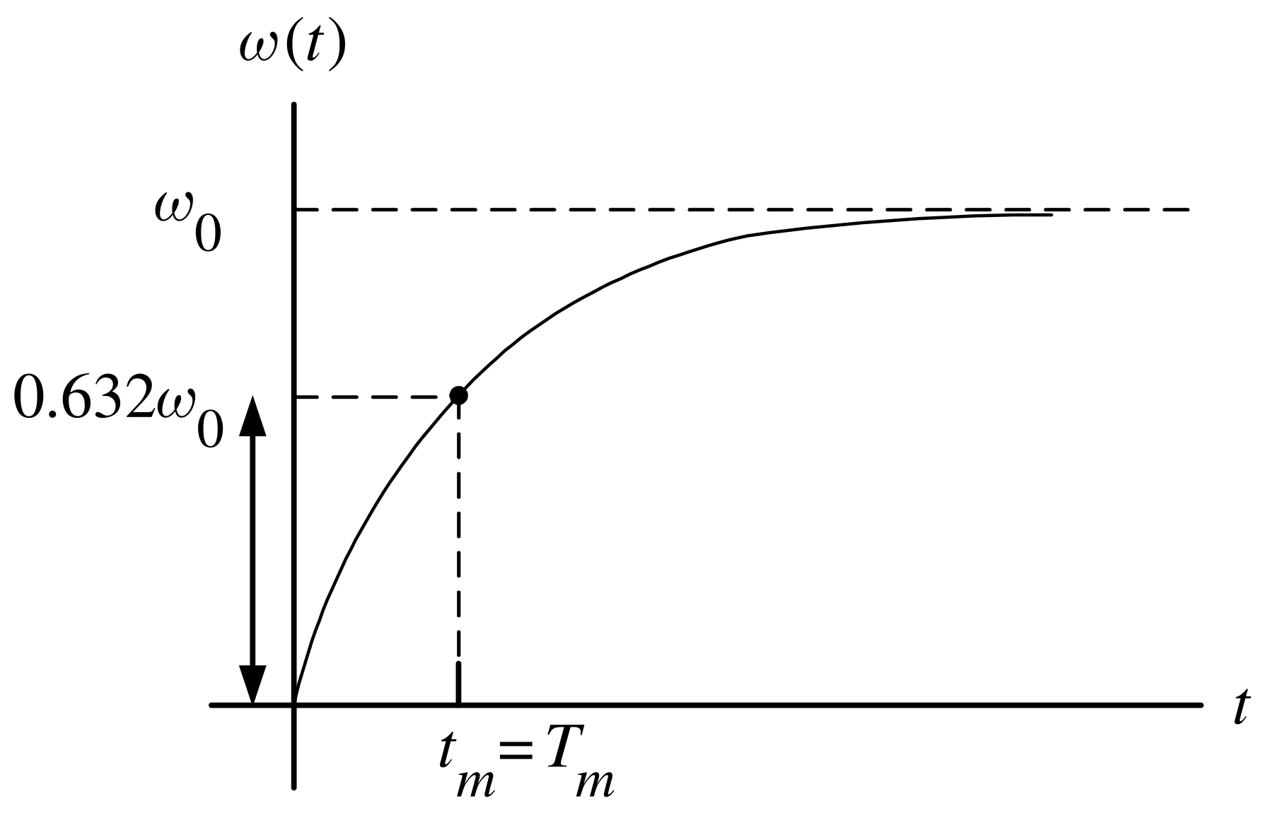
Identification of the Motor Transfer Function Model

Apply a constant voltage \(V_{0}\) to the motor and graph its speed \(\omega(t)\).
With \(\omega_{0}\) denoting the final speed we have \(K_{m}=\omega _{0}/V_{0}.\)
Measure the time \(t_{m}\) the speed reaches \(1-e^{-1}=0.632\) of its final value \(\omega_{0}.\)
Then \(T_{m}=t_{m}\).
The motor’s transfer function is \(G(s)=\dfrac{K_{m}}{T_{m}s+1}.\)
Or \(G(s)=\dfrac{b}{s+a}\) with \(a=1/T_{m}\) and \(b=K_{m}/T_{m}.\)

Second-Order Systems

Position Control of a DC Motor

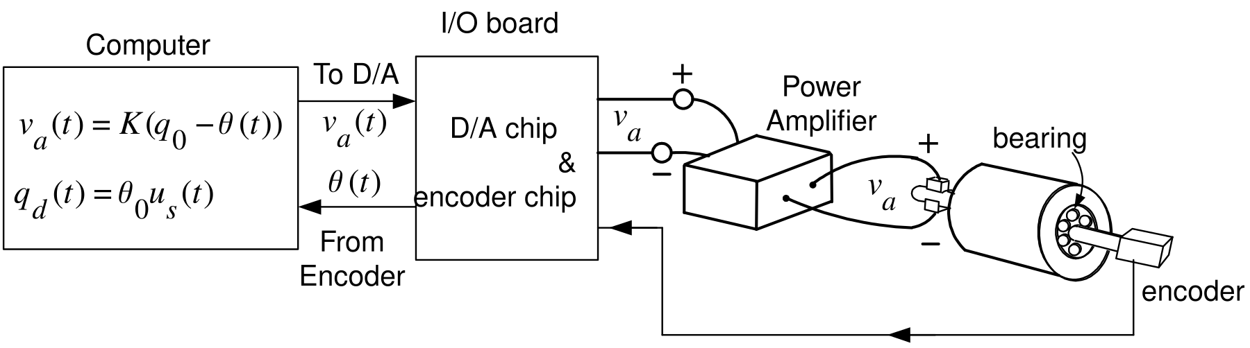
The computer reads in \(\theta(t)\) and sends out a value for \(v_{a}(t)\) to the D/A.

We want the motor rotate to the angle \(\theta_{0}\).

Let the reference (desired) motor angle be \(\theta_{d}(t)=\theta_{0}u_{s}(t).\)

Use proportional control, i.e., \(v_{a}(t)=K\!\left( \theta_{d}(t)-\theta(t)\right)\)

Block diagram model

\(a>0,b>0\) and \(K>0.\)

Position Control of a DC Motor

Standard notation \(R(s)=\theta_{d}(s)=R_{0}/s\) and \(C(s)=\theta(s)\).

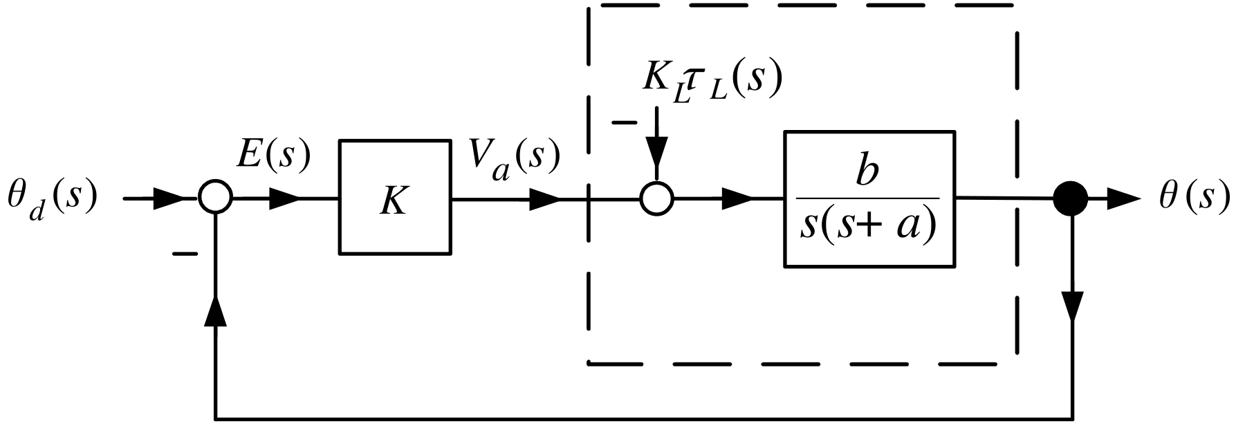
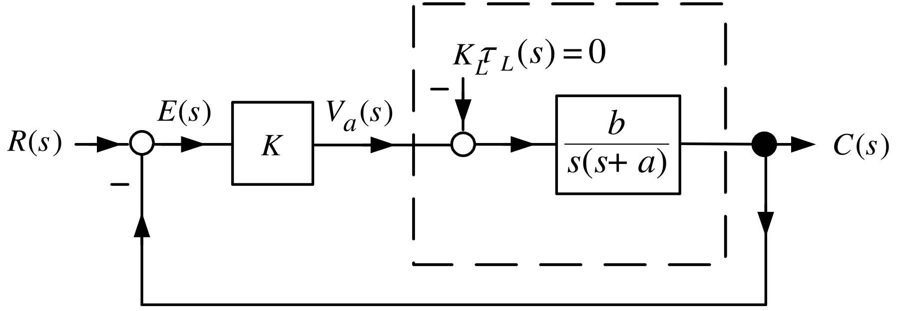
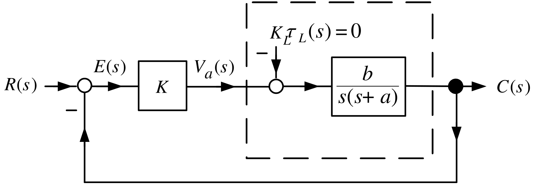
With \(\tau_{L}=0\) we have

\[ C(s)=\frac{\dfrac{bK}{s\left( s+a\right) }}{1+\dfrac{bK}{s\left( s+a\right) }}R(s)=\frac{bK}{s^{2}+as+bK}R(s). \]

Closed-loop transfer function

\[ \frac{C(s)}{R(s)}=\frac{bK}{s^{2}+as+bK} \]

With \(R(s)=R_{0}/s,\) set \(\omega_{n}^{2}\triangleq bK>0,\) and \(2\zeta\omega_{n}\triangleq a\) or \(\zeta\triangleq\dfrac{a}{2\omega_{n}}>0\).

\[ C(s)=\frac{\omega_{n}^{2}}{s^{2}+2\zeta\omega_{n}s+\omega_{n}^{2}}\frac{R_{0}}{s}. \]

\(\zeta\) is referred to as the damping ratio.

\(\omega_{n}\) is the natural frequency.

Position Control of a DC Motor

\(\zeta>0\) and \(\omega_{n}>0\) so that

\[ sC(s)=\frac{\omega_{n}^{2}}{s^{2}+2\zeta\omega_{n}s+\omega_{n}^{2}}R_{0} \]

is stable. By the FVT we have

\[ c(\infty)\triangleq\lim_{t\rightarrow\infty}c(t)=\lim_{s\rightarrow 0}sC(s)=\lim_{s\rightarrow0}s\frac{\omega_{n}^{2}}{s^{2}+2\zeta\omega _{n}s+\omega_{n}^{2}}\frac{R_{0}}{s}=R_{0}. \]

Thus \(c(t)\rightarrow R_{0}\) as \(t\rightarrow\infty.\)

Transient Response and Closed-Loop Poles

\[ C(s)=\underset{G(s)}{\underbrace{\frac{\omega_{n}^{2}}{s^{2}+2\zeta\omega _{n}s+\omega_{n}^{2}}}}\underset{\text{input}}{\underbrace{\frac{R_{0}}{s}}} \]

The poles of \(G(s)\) are the roots of \(s^{2}+2\zeta\omega_{n}s+\omega_{n}^{2}=0\):

\[ p_{i}=\frac{-2\zeta\omega_{n}\pm\sqrt{(2\zeta\omega_{n})^{2}-4\omega_{n}^{2}}}{2}=-\zeta\omega_{n}\pm\sqrt{(\zeta^{2}-1)\omega_{n}^{2}}=-\zeta\omega_{n}\pm\omega_{n}\sqrt{\zeta^{2}-1}. \]

Four cases:

\[ \begin{array} [c]{rll}0<\zeta<1 & & p_{1},p_{2}=-\zeta\omega_{n}\pm j\omega_{n}\sqrt{1-\zeta^{2}}\\ & & \\ \zeta=1 & & p_{1},p_{2}=-\omega_{n}\\ & & \\ \zeta>1 & & p_{1}=-\zeta\omega_{n}+\omega_{n}\sqrt{\zeta^{2}-1},\text{ }p_{2}=-\zeta\omega_{n}-\omega_{n}\sqrt{\zeta^{2}-1}\\ & & \\ \zeta=0 & & p_{1},p_{2}=\pm j\omega_{n}\end{array} \]

Both poles in the open LHP for \(\zeta>0\) making \(G(s)\) stable.
If \(\zeta=0\), then the poles are on the \(j\omega\) axis at \(\pm j\omega_{n}\).

Transient Response and Closed-Loop Poles

Pole locations for \(0<\zeta<1,\) \(p_{1},p_{2}=-\zeta\omega_{n}\pm j\omega_{n}\sqrt{1-\zeta^{2}}\)
\(\omega_{d}\triangleq\omega_{n}\sqrt{1-\zeta^{2}}\) is the damped frequency.

\[ \begin{aligned} \left\vert p_{i}\right\vert ^{2}=\left\vert -\zeta\omega_{n}\pm j\omega _{n}\sqrt{1-\zeta^{2}}\right\vert ^{2} & =(-\zeta\omega_{n})^{2}+\left( \pm\omega_{n}\sqrt{1-\zeta^{2}}\right) ^{2}\\ & =\zeta^{2}\omega_{n}^{2}+\omega_{n}^{2}(1-\zeta^{2})\\ & =\omega_{n}^{2}. \end{aligned} \]

For \(0\leq\zeta\leq1,\) poles are on a semicircle of radius of \(\omega_{n}\).
\(\tan(\phi)=\sqrt{1-\zeta^{2}}/\zeta\).

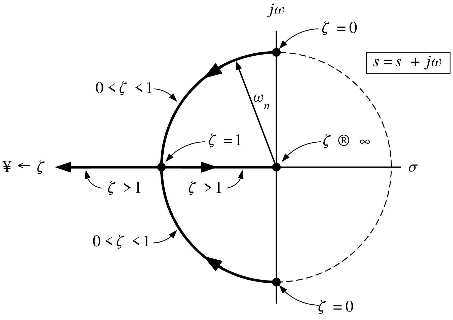
Transient Response and Closed-Loop Poles

\[ \begin{array} [c]{cl}0<\zeta<1 & p_{1},p_{2}=-\zeta\omega_{n}\pm j\omega_{n}\sqrt{1-\zeta^{2}}\\ & \\ \zeta=1 & p_{1},p_{2}=-\omega_{n}\\ & \\ \zeta>1 & p_{1}=-\zeta\omega_{n}+\omega_{n}\sqrt{\zeta^{2}-1},\text{ }p_{2}=-\zeta\omega_{n}-\omega_{n}\sqrt{\zeta^{2}-1}\\ & \\ \zeta=0 & p_{1},p_{2}=\pm j\omega_{n}\end{array} \]

Transient Response and Closed-Loop Poles

Consider \(0<\zeta<1\) so \(p_{1},p_{2}=-\zeta\omega_{n}\pm j\omega_{n}\sqrt{1-\zeta^{2}}.\)

\[ \begin{aligned} C(s) & =\frac{\omega_{n}^{2}}{s^{2}+2\zeta\omega_{n}s+\omega_{n}^{2}}\frac{R_{0}}{s}\\ & =\frac{\omega_{n}^{2}}{\left( s-(-\zeta\omega_{n}+j\omega_{n}\sqrt {1-\zeta^{2}})\right) \!\left( s-(-\zeta\omega_{n}-j\omega_{n}\sqrt {1-\zeta^{2}})\right) }\frac{R_{0}}{s}\\ & =\frac{R_{0}}{s}+\frac{\beta}{s-(-\zeta\omega_{n}+j\omega_{n}\sqrt {1-\zeta^{2}})}+\frac{\beta^{\ast}}{s-(-\zeta\omega_{n}-j\omega_{n}\sqrt{1-\zeta^{2}})}.\\ & \\ & \\ \text{So }c(t) & =R_{0}u_{s}(t)+\beta e^{-\zeta\omega_{n}t}e^{+j\omega _{n}\sqrt{1-\zeta^{2}}t}+\beta^{\ast}e^{-\zeta\omega_{n}t}e^{-j\omega_{n}\sqrt{1-\zeta^{2}}t}\\ & \\ & =R_{0}u_{s}(t)+2|\beta|e^{-\zeta\omega_{n}t}\!\cos\!\left( \!\omega _{n}\sqrt{1-\zeta^{2}}t+\angle\beta\right) . \end{aligned} \]

Transient dies out according to the real part \(-\zeta\omega_{n}\) of the poles.
Typically want \(0.6\leq\zeta\leq0.8\)

Transient Response and Closed-Loop Poles

Compute \(c(t)\):

\[ \begin{aligned} C(s) & =\frac{\omega_{n}^{2}}{s^{2}+2\zeta\omega_{n}s+\omega_{n}^{2}}\frac{R_{0}}{s}=\frac{R_{0}}{s}+\frac{A_{1}(s+\zeta\omega_{n})+A_{2}\omega _{n}\sqrt{1-\zeta^{2}}}{(s+\zeta\omega_{n})^{2}+\omega_{n}^{2}(1-\zeta^{2})}.\\ \Longrightarrow\text{ }\omega_{n}^{2}R_{0} & =\left( s^{2}+2\zeta \omega_{n}s+\omega_{n}^{2}\right) \!R_{0}+s\!\left( \!A_{1}(s+\zeta\omega_{n})+A_{2}\omega_{n}\sqrt{1-\zeta^{2}}\!\right) \end{aligned} \]

Equating powers of \(s\):

\[ \begin{array} [c]{cl}s^{2} & 0=(R_{0}+B)s^{2}\Longrightarrow A_{1}=-R_{0}\\ s^{1} & 0=\left( 2\zeta\omega_{n}R_{0}+A_{1}\zeta\omega_{n}+A_{2}\omega _{n}\sqrt{1-\zeta^{2}}\right) \!s\Longrightarrow A_{2}=-R_{0}\zeta /\sqrt{1-\zeta^{2}}\\ s^{0} & \omega_{n}^{2}R_{0}=\omega_{n}^{2}R_{0}\end{array} \]

Then

\[ C(s)=\frac{R_{0}}{s}-R_{0}\frac{s+\zeta\omega_{n}}{(s+\zeta\omega_{n})^{2}+\omega_{n}^{2}(1-\zeta^{2})}-\frac{R_{0}\zeta}{\sqrt{1-\zeta^{2}}}\frac{\omega_{n}\sqrt{1-\zeta^{2}}}{(s+\zeta\omega_{n})^{2}+\omega_{n}^{2}(1-\zeta^{2})} \]

Transient Response and Closed-Loop Poles

From previous slide:

\[ \begin{aligned} e^{\sigma t}\sin(\omega t)u_{s}(t) & \leftrightarrow\frac{\omega}{(s-\sigma)^{2}+\omega^{2}}\\ e^{\sigma t}\cos(\omega t)u_{s}(t) & \leftrightarrow\frac{s-\sigma}{(s-\sigma)^{2}+\omega^{2}}. \end{aligned} \]

For \(t>0\) we have

\[ \begin{aligned} c(t) & =R_{0}-R_{0}e^{-\zeta\omega_{n}t}\cos\!\left( \omega_{n}\sqrt {1-\zeta^{2}}t\right) -R_{0}\frac{\zeta}{\sqrt{1-\zeta^{2}}}e^{-\zeta\omega_{n}t}\sin\!\left( \omega_{n}\sqrt{1-\zeta^{2}}t\right) \\ & =R_{0}-R_{0}\frac{e^{-\zeta\omega_{n}t}}{\sqrt{1-\zeta^{2}}}\left( \sqrt{1-\zeta^{2}}\cos\!\left( \omega_{n}\sqrt{1-\zeta^{2}}t\right) +\right. \left. \zeta\sin\!\left( \omega_{n}\sqrt{1-\zeta^{2}}t\right) \right) \\ & =R_{0}-R_{0}\frac{e^{-\zeta\omega_{n}t}}{\sqrt{1-\zeta^{2}}}\left( \sin\left( \phi\right) \cos\!\left( \omega_{n}\sqrt{1-\zeta^{2}}t\right) +\right. \left. \cos\left( \phi\right) \sin\!\left( \omega_{n}\sqrt{1-\zeta^{2}}t\right) \right) \\ & =R_{0}-R_{0}\frac{e^{-\zeta\omega_{n}t}}{\sqrt{1-\zeta^{2}}}\sin\!\left( \omega_{n}\sqrt{1-\zeta^{2}}t+\phi\right) \end{aligned} \]

where \(\sin\left( \phi\right) \triangleq\sqrt{1-\zeta^{2}},\) \(\cos\left( \phi\right) \triangleq\zeta\) so \(\phi\triangleq\tan^{-1}\!\left( \dfrac{\sqrt{1-\zeta^{2}}}{\zeta}\right) .\)

Transient Response and Closed-Loop Poles

\[ c(t)=R_{0}u_{s}(t)-R_{0}\frac{e^{-\zeta\omega_{n}t}}{\sqrt{1-\zeta^{2}}}\sin\!\left( \omega_{n}\sqrt{1-\zeta^{2}}t+\phi\right) \!u_{s}(t)\text{ for }0<\zeta<1 \]

Peak Time t_p

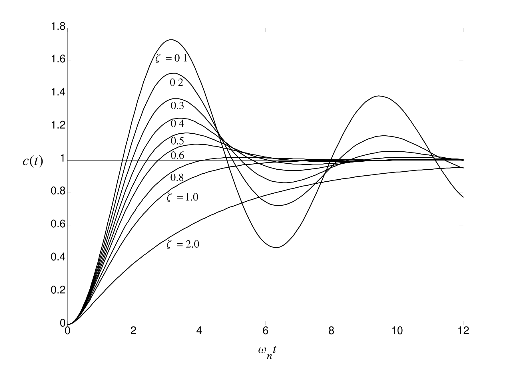
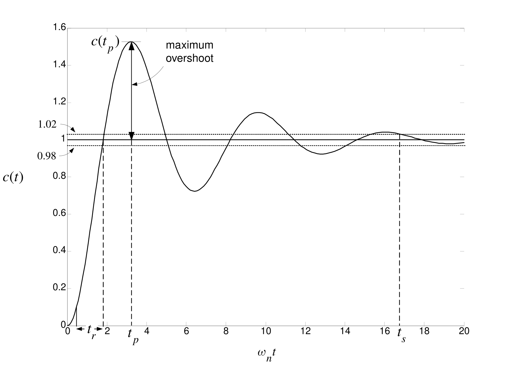
For \(0<\zeta<1\) the output response is oscillatory with frequency \(\omega _{d}=\omega_{n}\sqrt{1-\zeta^{2}}\).

We next compute the peak time \(t_{p}\) and the peak value \(c(t_{p})\).

Peak Time t_p and Peak Value c(t_p)

\[ \begin{aligned} c(t) & =R_{0}-R_{0}e^{-\zeta\omega_{n}t}\cos\!\left( \!\omega_{n}\sqrt{1-\zeta^{2}}t\!\right) -R_{0}\frac{\zeta}{\sqrt{1-\zeta^{2}}}e^{-\zeta\omega_{n}t}\sin\!\left( \!\omega_{n}\sqrt{1-\zeta^{2}}t\!\right) \\ & =R_{0}-R_{0}e^{\sigma t}\cos\left( \omega_{d}t\right) +R_{0}\frac{\sigma }{\omega_{d}}e^{\sigma t}\sin\left( \omega_{d}t\right) \text{ where }\sigma=-\zeta\omega_{n}. \end{aligned} \]

Differentiate:

\[ \begin{aligned} \!\!\!\!\!\frac{d}{dt}c(t)\!\!\!\! & =\!\!\!\!-R_{0}\sigma e^{\sigma t}\cos(\omega_{d}t)+R_{0}\omega_{d}e^{\sigma t}\sin(\omega_{d}t)+R_{0}\frac{\sigma^{2}}{\omega_{d}}e^{\sigma t}\sin(\omega_{d}t)+R_{0}\sigma e^{\sigma t}\cos(\omega_{d}t)\\ & =R_{0}e^{\sigma t}\!\left( \frac{\sigma^{2}}{\omega_{d}}+\omega_{d}\right) \!\sin\left( \omega_{d}t\right) . \end{aligned} \]

\(\dfrac{d}{dt}c(t)=0\) \(\Longrightarrow\) \(\sin\left( \omega_{d}t_{p}\right) =0\) or

\[ t_{p}=\frac{\pi}{\omega_{d}}=\frac{\pi}{\omega_{n}\sqrt{1-\zeta^{2}}}\text{ }\left( \Longrightarrow\sigma t_{p}=-\pi\zeta/\sqrt{1-\zeta^{2}}\right) . \]

The value of \(c(t)\) at \(t_{p}\) is

\[ \begin{aligned} \!\!\!\!\!\!\!\!c(t_{p})=R_{0}-R_{0}e^{\sigma t_{p}}\cos(\omega_{d}t_{p})+R_{0}\frac{\sigma}{\omega_{d}}e^{\sigma t_{p}}\sin(\omega_{d}t_{p})\!\!\! & =\!\!\!\!\!\!R_{0}-R_{0}e^{\sigma t_{p}}\cos(\pi)\\ \!\!\!\! & =\!\!\!\!\!\!R_{0}+R_{0}e^{-\pi\zeta/\!\!\!\sqrt{1-\zeta^{2}}}\!. \end{aligned} \]

Percent Overshoot M_p

We just showed

\[ t_{p}=\frac{\pi}{\omega_{d}}=\frac{\pi}{\omega_{n}\sqrt{1-\zeta^{2}}}. \]

and

\[ \begin{aligned} c(t_{p})=R_{0}-R_{0}e^{\sigma t_{p}}\cos(\omega_{d}t_{p})+R_{0}\frac{\sigma }{\omega_{d}}e^{\sigma t_{p}}\sin(\omega_{d}t_{p}) & =R_{0}-R_{0}e^{\sigma t_{p}}\cos(\pi)\\ & =R_{0}+R_{0}e^{-\pi\zeta/\sqrt{1-\zeta^{2}}}. \end{aligned} \]

Fractional Overshoot \(M_{p}:\)

\[ M_{p}\triangleq\frac{c(t_{p})-c(\infty)}{c(\infty)}=\frac{(R_{0}+R_{0}e^{-\pi\zeta/\sqrt{1-\zeta^{2}}})-R_{0}}{R_{0}}=e^{-\pi\zeta/\sqrt{1-\zeta ^{2}}} \]

The Percent Overshoot is \(100\times M_{p}=100e^{-\pi\zeta /\sqrt{1-\zeta^{2}}}.\)

Identification of Motor Parameters \(G(s)=\dfrac {b}{s(s+a)}\)

From previous slide:

\[ M_{p}\triangleq\frac{c(t_{p})-c(\infty)}{c(\infty)}=e^{-\pi\zeta/\sqrt {1-\zeta^{2}}} \]

From the step response measure \(t_{p}\) and \(c(t_{p}).\)

Compute \(M_{p}\triangleq\dfrac{c(t_{p})-c(\infty)}{c(\infty)}.\)

Compute \(\zeta\) as follows:

\[ \begin{aligned} \ln(M_{p})=-\pi\zeta/\sqrt{1-\zeta^{2}} & \Longrightarrow(1-\zeta^{2})\ln ^{2}(M_{p})=\pi^{2}\zeta^{2}\\ & \Longrightarrow\text{ }\zeta=\sqrt{\frac{\ln^{2}(M_{p})}{\pi^{2}+\ln ^{2}(M_{p})}}. \end{aligned} \]

Compute \(\omega_{n}\) as follows:

\[ \begin{aligned} t_{p} & =\frac{\pi}{\omega_{n}\sqrt{1-\zeta^{2}}}\\ \Longrightarrow\text{ }\omega_{n} & =\frac{\pi}{t_{p}\sqrt{1-\zeta^{2}}}. \end{aligned} \]

Identification of Motor Parameters \(G(s)=\dfrac{b}{s(s+a)}\)

From previous slide:

\[ \zeta=\sqrt{\frac{\ln^{2}(M_{p})}{\pi^{2}+\ln^{2}(M_{p})}}\text{ and }\omega_{n}=\frac{\pi}{t_{p}\sqrt{1-\zeta^{2}}} \]

\[ C(s)=\frac{Kb}{s^{2}+as+Kb}\frac{R_{0}}{s}=\frac{\omega_{n}^{2}}{s^{2}+2\zeta\omega_{n}s+\omega_{n}^{2}}\frac{R_{0}}{s} \]

we have

\[ \begin{aligned} Kb & =\omega_{n}^{2}\\ & \\ a & =2\zeta\omega_{n}. \end{aligned} \]

Motor Parameters:

\[ \begin{aligned} b & =\omega_{n}^{2}/K\\ & \\ a & =2\zeta\omega_{n}. \end{aligned} \]

Settling Time t_s

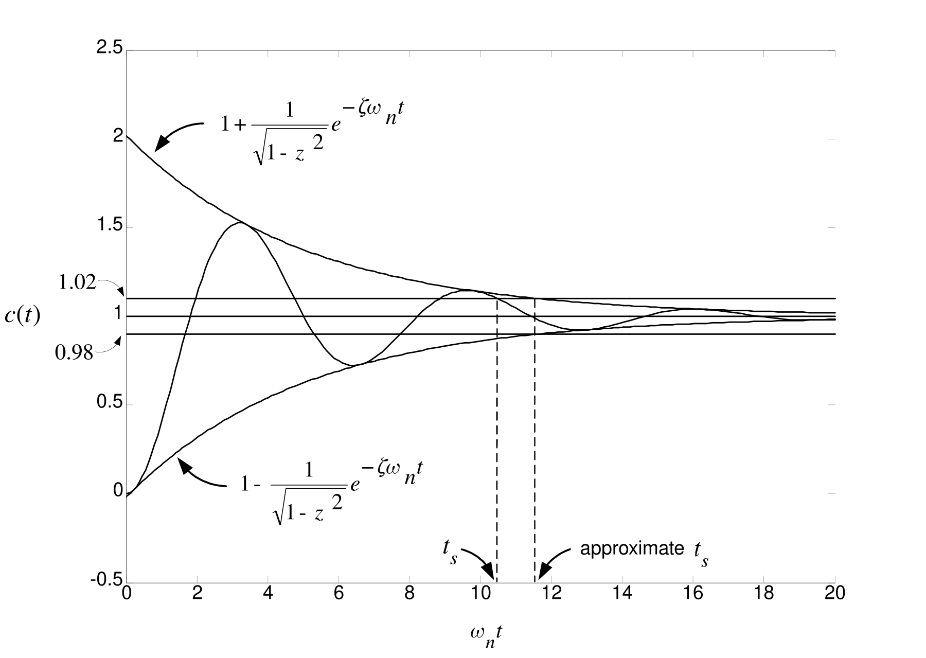
\(t_{s}\): The first time \(c(t)\) stays within \(2\%\) of its final value.
\(t_{s}\) approximation: Compute the time the envelope of \(c(t)\) intersects \((1\pm0.02)R_{0}\).

Settling Time t_s

\[ c(t)=R_{0}u_{s}(t)-R_{0}\frac{e^{-\zeta\omega_{n}t}}{\sqrt{1-\zeta^{2}}}\sin\!\left( \omega_{n}\sqrt{1-\zeta^{2}}t+\phi\right) u_{s}(t). \]

The envelope of \(c(t)\) is given by

\[ R_{0}\pm R_{0}\frac{e^{-\zeta\omega_{n}t}}{\sqrt{1-\zeta^{2}}} \]

An an upper bound \(t_{sb}\) on the settling time \(t_{s}\) is a solution to

\[ R_{0}+R_{0}\frac{e^{-\zeta\omega_{n}t_{sb}}}{\sqrt{1-\zeta^{2}}}=1.02R_{0}. \]

Solve for \(t_{sb}\) as follows.

\[ \frac{e^{-\zeta\omega_{n}t_{sb}}}{\sqrt{1-\zeta^{2}}}=0.02\text{ or }e^{-\zeta\omega_{n}t_{sb}}=0.02\sqrt{1-\zeta^{2}}\text{ or }-\zeta\omega_{n}t_{sb}=\ln\!\left( 0.02\sqrt{1-\zeta^{2}}\right) \!. \]

Finally

\[ t_{s}\leq t_{sb}=-\frac{\ln\!\left( 0.02\sqrt{1-\zeta^{2}}\right) }{\zeta\omega_{n}}. \]

Settling Time

\(t_{s}\)

From previous slide:

\[ t_{s}\leq t_{sb}=-\frac{\ln\!\left( 0.02\sqrt{1-\zeta^{2}}\right) }{\zeta\omega_{n}}. \]

The envelope approach gives an upper bound for the settling time.
\(t_{sb}\) goes to \(+\infty\) as either \(\zeta\rightarrow1\) or as \(\zeta\rightarrow0\).

\(\Longrightarrow\) \(t_{sb}\) is not a useful approximation for these two cases.
We want the overshoot to be small which means \(\zeta\) is close to \(1.\)
Often in textbooks they set \(\sqrt{1-\zeta^{2}}\approx1\) (implying \(\zeta\) small!) to obtain

\[ t_{s}\leq t_{sb}\approx-\frac{\ln(0.02)}{\zeta\omega_{n}}\approx\dfrac {4}{\zeta\omega_{n}}. \]

Different Approach to Defining t_s

Take \(\zeta=1\) so there is no overshoot.
\(C(s)=\dfrac{\omega_{n}^{2}}{s^{2}+2\zeta\omega_{n}s+\omega_{n}^{2}}\dfrac{R_{0}}{s}=\dfrac{\omega_{n}^{2}}{(s+\omega_{n})^{2}}\dfrac{R_{0}}{s}=\dfrac{1}{s}R_{0}-\dfrac{R_{0}}{s+\omega_{n}}-\omega_{n}\dfrac{R_{0}}{\left( s+\omega_{n}\right) ^{2}}.\)
\(c(t)=R_{0}-R_{0}(e^{-t\omega_{n}}+t\omega_{n}e^{-t\omega_{n}}).\)
At \(t=\left. \dfrac{4}{\zeta\omega_{n}}\right\vert _{\zeta=1}=\dfrac {4}{\omega_{n}}\):

\[ e^{-t_{s}\omega_{n}}+t_{s}\omega_{n}e^{-t_{s}\omega_{n}}=e^{-4}+4e^{-4}=5e^{-4}=0.092\approx0.1 \]

\(c(t)\) is within \(10\%\) of the final value \(R_{0}\) (rather than \(2\%\)).
Define \(t_{s}\triangleq\dfrac{4}{\zeta\omega_{n}}\) even if \(\zeta\) is not 1.
Define the time constant of the complex-conjugate pair of closed-loop poles by

\[ \left\vert \dfrac{1}{\sigma}\right\vert =\left\vert \dfrac{1}{-\zeta\omega _{n}}\right\vert =\dfrac{1}{\zeta\omega_{n}}. \]

\(t_{s}\) is defined to be four time constants long.
The further in the LHP the CLPs are located, the faster the transients die out and thus the faster the system reaches its final value.

Rise Time

\(t_{r}\)

\(t_{r}\) is the amount of time for \(c(t)\) to go from \(0.1R_{0}\) to the first time it reaches \(R_{0}\).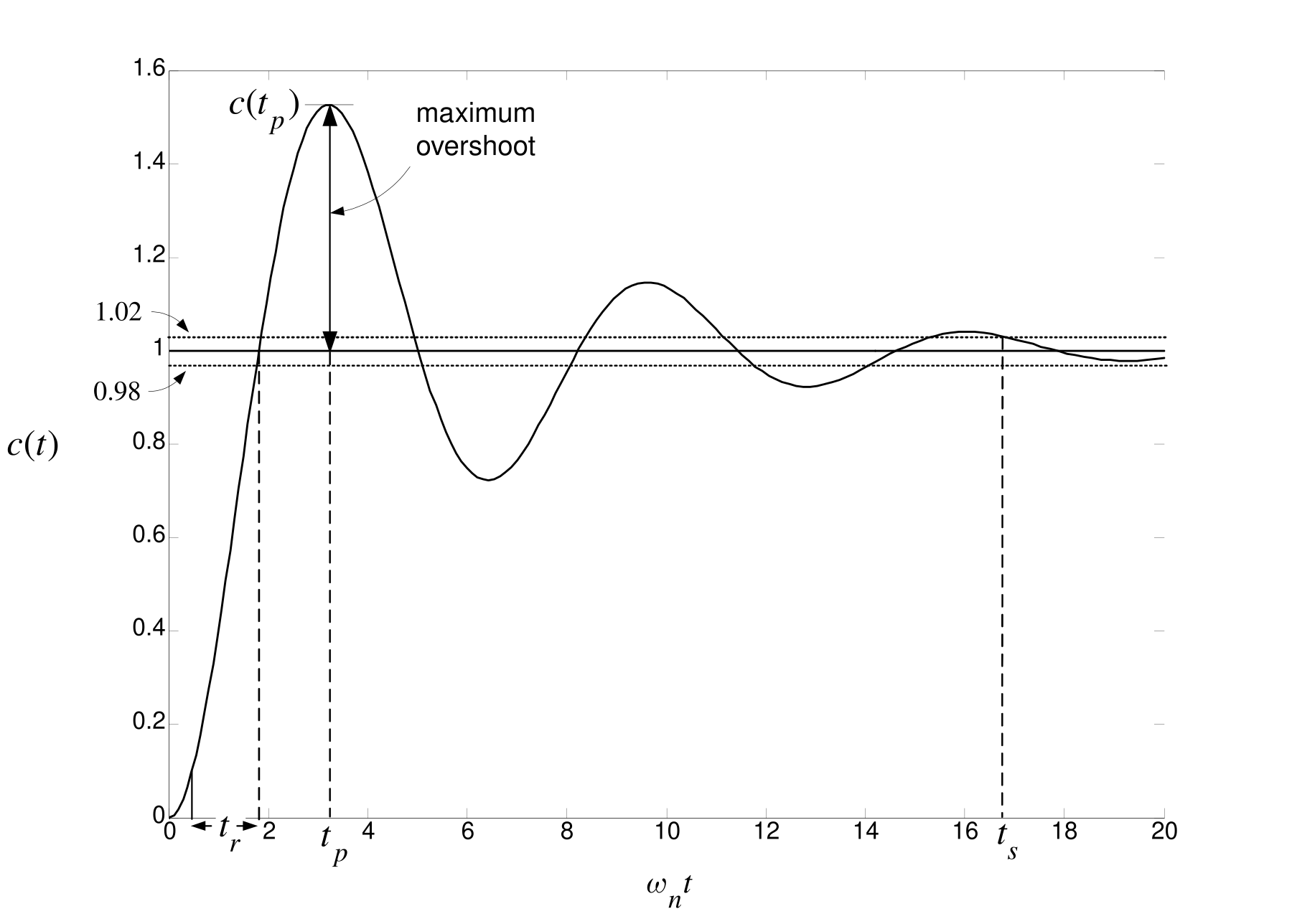

Note: For \(\zeta<0.5,\) \(c(t)=0.1R_{0}\) at \(\omega_{n}t\approx0.2\) and \(c(t)=R_{0}\) at \(\omega_{n}t\approx2.\)

Rise Time

\(t_{r}\)

Typical textbook approximation: For \(\zeta<0.5\)

\[ \begin{aligned} c(t_{1}) & =0.1R_{0}\text{ at }\omega_{n}t_{1}\approx0.2\\ & \\ c(t_{2}) & =R_{0} \text{ at }\omega_{n}t_{2}\approx2. \end{aligned} \]

Then

\[ t_{r}=t_{2}-t_{1}\approx\frac{2-0.2}{\omega_{n}}=\frac{1.8}{\omega_{n}}. \]

Not very useful as we want \(\zeta\) to be close to 1 to have small overshoot!

Summary of

\(M_{p},t_{p},t_{s}\)

Second-order system with a step input:

\[ C(s)=\dfrac{\omega_{n}^{2}}{s^{2}+2\zeta\omega_{n}s+\omega_{n}^{2}}\dfrac{R_{0}}{s}. \]

Then

\[ \begin{aligned} M_{p} & \triangleq\frac{c(t_{p})-c(\infty)}{c(\infty)}=e^{-\pi\zeta /\sqrt{1-\zeta^{2}}}\text{ with }t_{p}=\frac{\pi}{\omega_{n}\sqrt {1-\zeta^{2}}}\\ & \\ t_{s} & =\frac{4}{\zeta\omega_{n}},\dfrac{5}{\zeta\omega_{n}},\dfrac{6}{\zeta\omega_{n}}\text{ for }10\%,4\%,2\%\text{ of the final value and }\zeta\text{ close to 1.}\\ & \\ t_{r} & =\frac{1.8}{\omega_{n}}\text{ for }\zeta<0.5. \end{aligned} \]

In general, we are concerned about overshoot, settling time, and rise time.
However, these expressions are only valid for 2\(^{nd}\)-order systems with no zeros.

Choosing the Gain K of a Proportional Controller

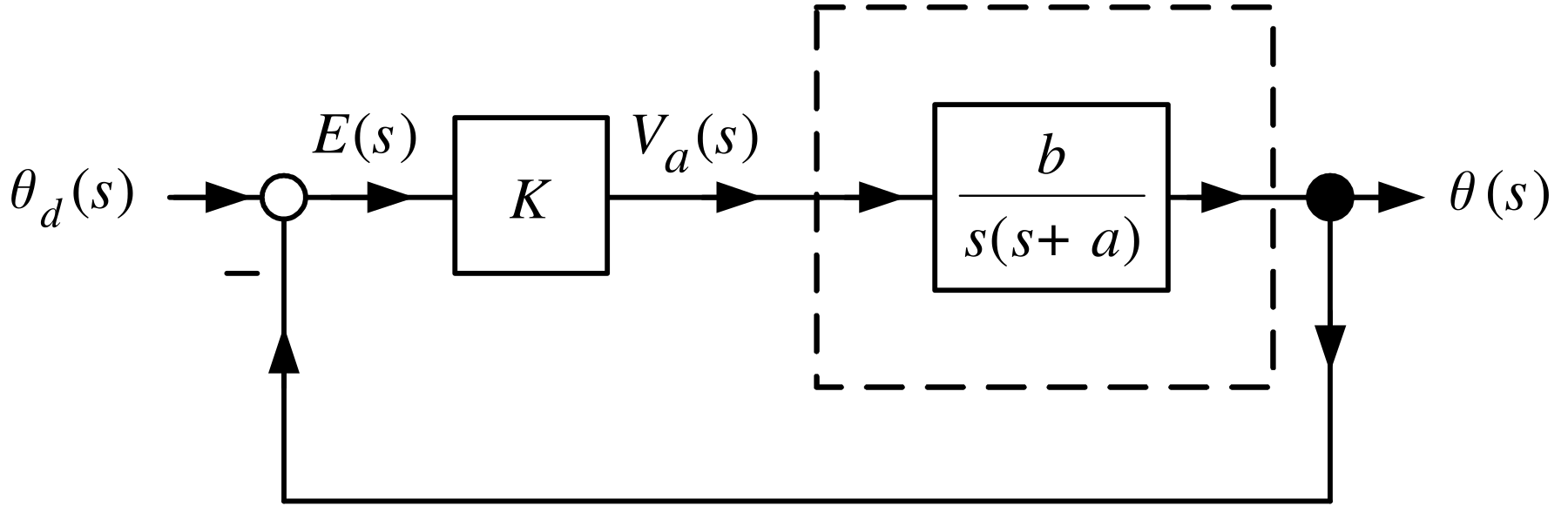
\[ \frac{\theta(s)}{\theta_{d}(s)}=\frac{K\dfrac{b}{s(s+a)}}{1+K\dfrac{b}{s(s+a)}}=\frac{Kb}{s^{2}+as+Kb}. \]

Let \(b=1,\) \(a=4\), and \(\theta_{d}(s)=\dfrac{\theta_{0}}{s}\) so

\[ \theta(s)=\frac{K}{s^{2}+4s+K}\frac{\theta_{0}}{s}. \]

For \(K>0\) the quadratic formula shows the roots of \(s^{2}+4s+K\) are in the open LHP.

Thus \(s\theta(s)=\dfrac{K}{s^{2}+4s+K}\theta_{0}\) is stable.

By the FVT

\[ \theta(\infty)=\lim_{t\rightarrow\infty}\theta(t)=\lim_{s\rightarrow0}s\theta(s)=\theta_{0}. \]

Choosing the Gain K of a Proportional Controller

The behavior of the \(\theta(t)\) as it goes to \(\theta_{0}\) is determined by the location of the CLPs.

Need to find the pole locations as \(K\) is varied from \(0\) to \(\infty\).

Solving \(s^{2}+4s+K=0\) gives

\[ s=\frac{-4\pm\sqrt{16-4K}}{2}=-2\pm\sqrt{4-K}. \]

The closed-loop poles are

\[ p_{i}=\left\{ \begin{array} [c]{cl}-2\pm\sqrt{4-K}, & 0\leq K\leq4\\ -2\pm j\sqrt{K-4}, & 4<K. \end{array} \right. \]

\[ \begin{array}{c|l} \hline K & \text{Closed-Loop Poles}\\\hline 0 & s=0,-4\\\hline 2 & s=-2\pm\sqrt{2}=-3.414,-0.596\\\hline 4 & s=-2,-2\\\hline 8 & s=-2\pm2j\\\hline 13 & s=-2\pm3j\\\hline \end{array} \]

Choosing the Gain K of a Proportional Controller

Root Locus: Sketch of the closed-loop poles as \(K\) varies.

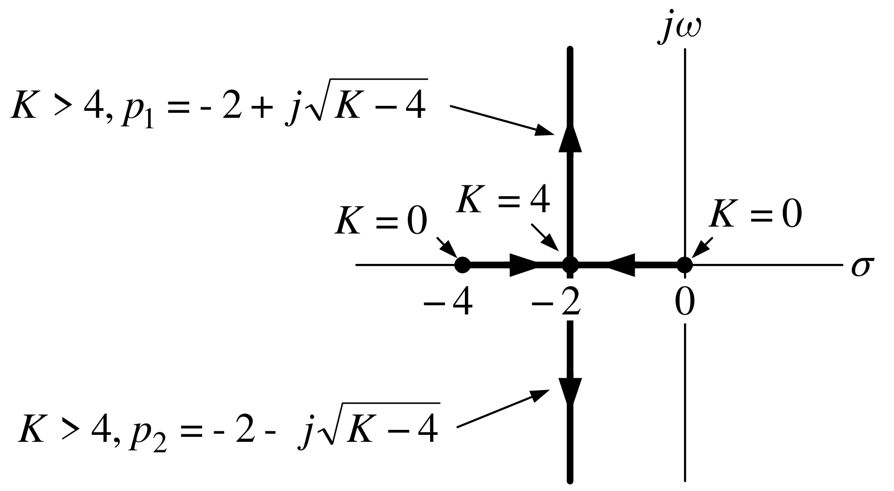
Both poles are in the open left half-plane for \(K>0.\)
For \(K>4\), complex conjugate closed-loop poles result in an oscillatory response.
Want poles as far in the LHP as possible so take \(K\geq4\).
Don’t take \(K\) too large as this would command a large voltage to the amplifier.

Root Locus Computation

% RootLocus_G(s) = K*b/(s2+a*s)

% G_cl(s) = KG(s)/(1 + KG(s)) = Kb/(s2 + as + Kb)

close all; clear; clc

%

a = 4;b = 1;

% Open loop transfer function G(s) = b/(s*(s+a)) = b/(s2+a*s)

den = [1 a 0]; num = [b]; tf_openloop = tf(num,den);

%

% Plot the CLPs for K going from 0 to 100 in steps of 1.

K = [0:1:100]; rlocus(tf_openloop,K)

%

% Make the linewidth thicker, the marker size and font size bigger.

h = findobj(gca, ’Type’, ’line’);

set(h, ’LineWidth’, 4); set(h, ’MarkerSize’, 15); set(gca,’FontSize’,20)

%

% Set range of x-axis [-5,0] and y-axis [-10,10]

v = [-5 0 -10 10]; axis(v);

%

title(’G(s)= b/(s2+as)’,’FontSize’,20)

xlabel(’Re(s)’,’FontSize’,20); ylabel (’Im(s)’,’FontSize’,20)

%

K = 6.25; p = rlocus(num,den,K) % Gives the CLP for this value of K

Choosing the Gain K of a Proportional Controller

Choose \(K\) so the damping ratio \(\zeta\) is \(0.8\).

\[ \theta(s)=\frac{K}{s^{2}+4s+K}\frac{\theta_{0}}{s}=\frac{\omega_{n}^{2}}{s^{2}+2\zeta\omega_{n}s+\omega_{n}^{2}}\frac{\theta_{0}}{s} \]

Equate coefficients:

\[ \begin{aligned} s^{2}+4s+K & =s^{2}+2\zeta\omega_{n}s+\omega_{n}^{2}\\ \Longrightarrow4 & =2\zeta\omega_{n},\text{ }K=\omega_{n}^{2}\\ \Longrightarrow K & =\left. \left( \frac{4}{2\zeta}\right) ^{2}\right\vert _{\zeta=0.8}=6.25. \end{aligned} \]

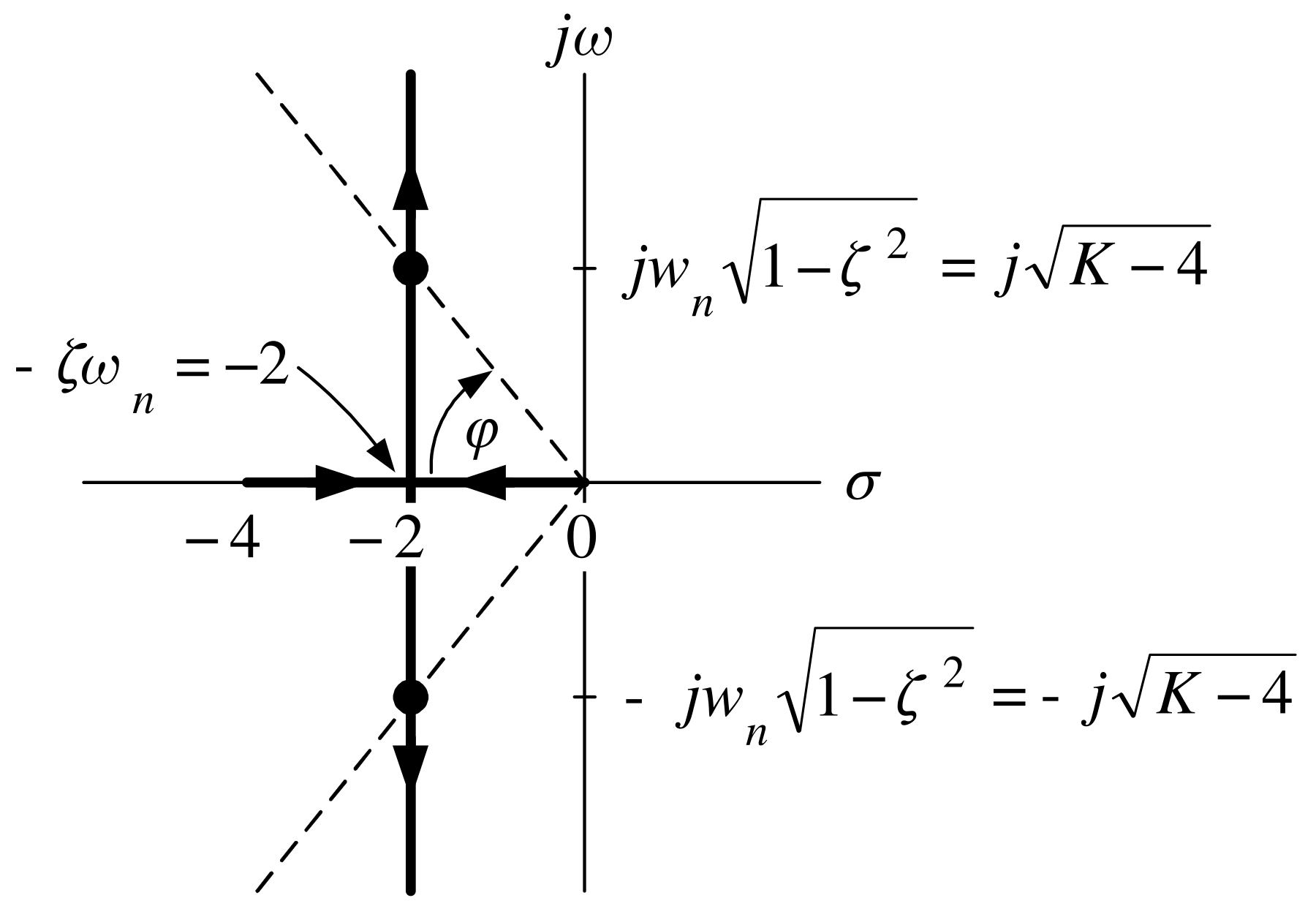
Choosing the Gain K of a Proportional Controller - Geometric View

\[ \begin{aligned} s^{2}+4s+K & =s^{2}+2\zeta\omega_{n}s+\omega_{n}^{2}\\ \Longrightarrow s & =-2\pm j\sqrt{K-4}\\ & =-\zeta\omega_{n}\pm j\omega_{n}\sqrt{1-\zeta^{2}} \end{aligned} \]

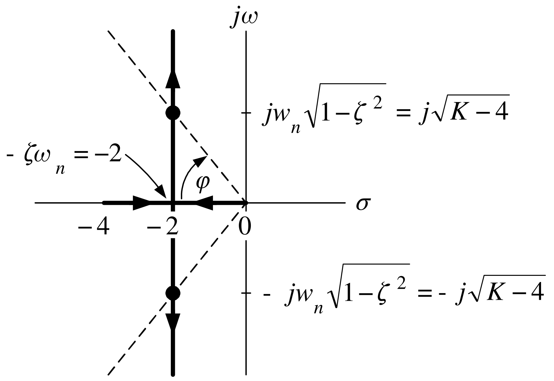
\[ \begin{aligned} \tan(\phi) & =\dfrac{\omega_{n}\sqrt{1-\zeta^{2}}}{\zeta\omega_{n}}=\dfrac{\sqrt{K-4}}{2}\\ \Longrightarrow K & =4\dfrac{1-\zeta^{2}}{\zeta^{2}}+4=\dfrac{4}{\zeta^{2}}=\dfrac{4}{0.64}=6.25. \end{aligned} \]

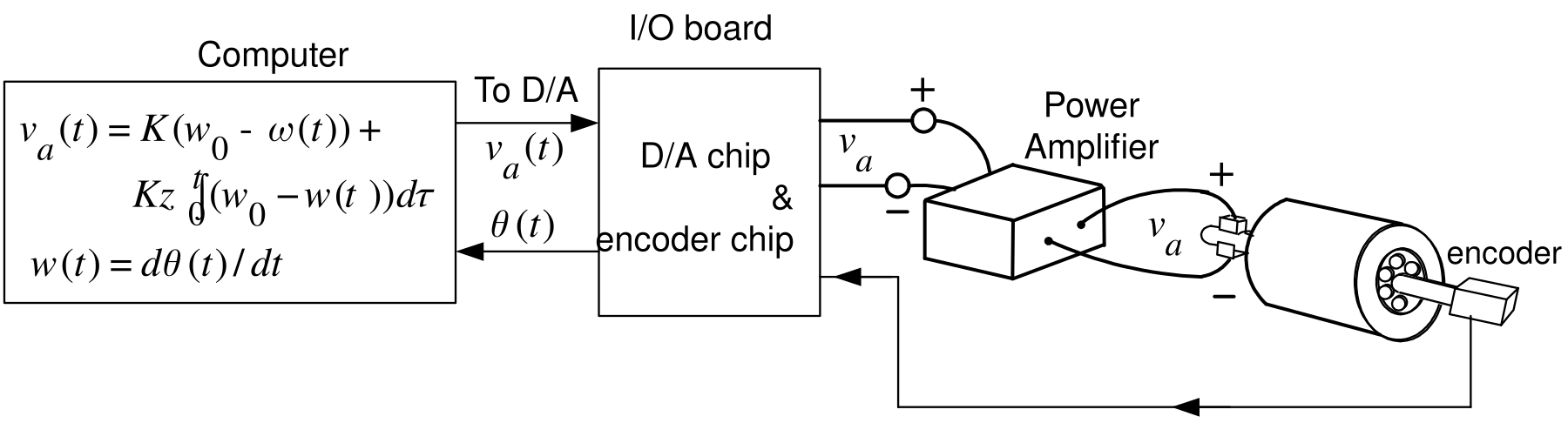
Second-Order Systems with Zeros Example Speed Control of a DC Motor

\(\omega(t)\) is found by numerically differentiating the measured \(\theta(t).\)
The controller is \(v_{a}(t)=K(\omega_{0}-\omega(t))+Kz\int_{0}^{t}(\omega_{0}-\omega(\tau))d\tau\).
\(\omega_{0}\) is the desired speed.
\(E(s)=\dfrac{\omega_{0}}{s}-\omega(s)\) and \(V_{a}(s)=KE(s)+Kz\dfrac {1}{s}E(s)=K\dfrac{s+z}{s}E(s).\)
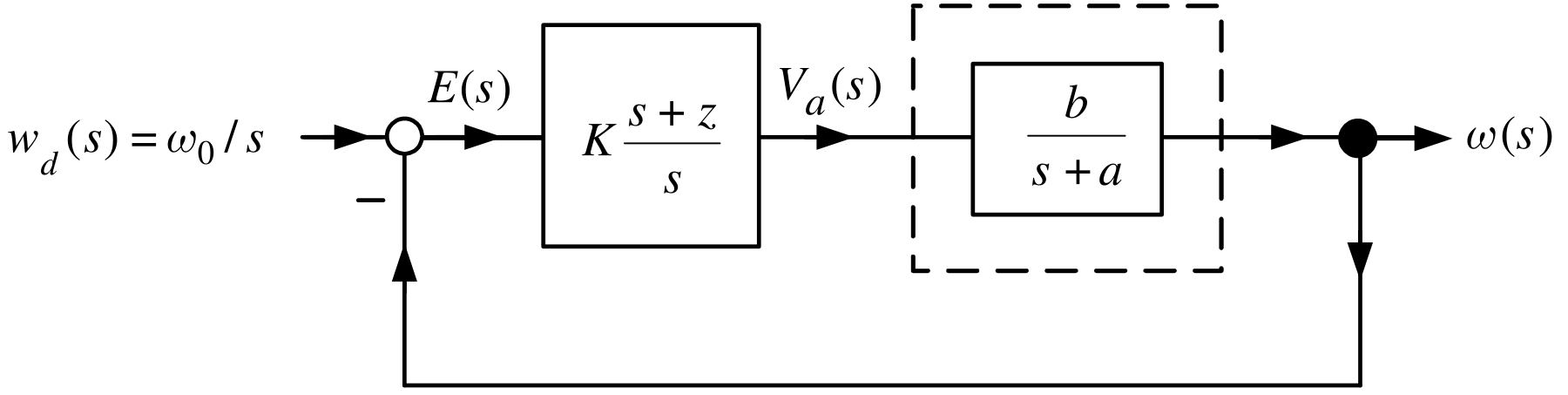
This is a proportional plus integral (PI) controller.

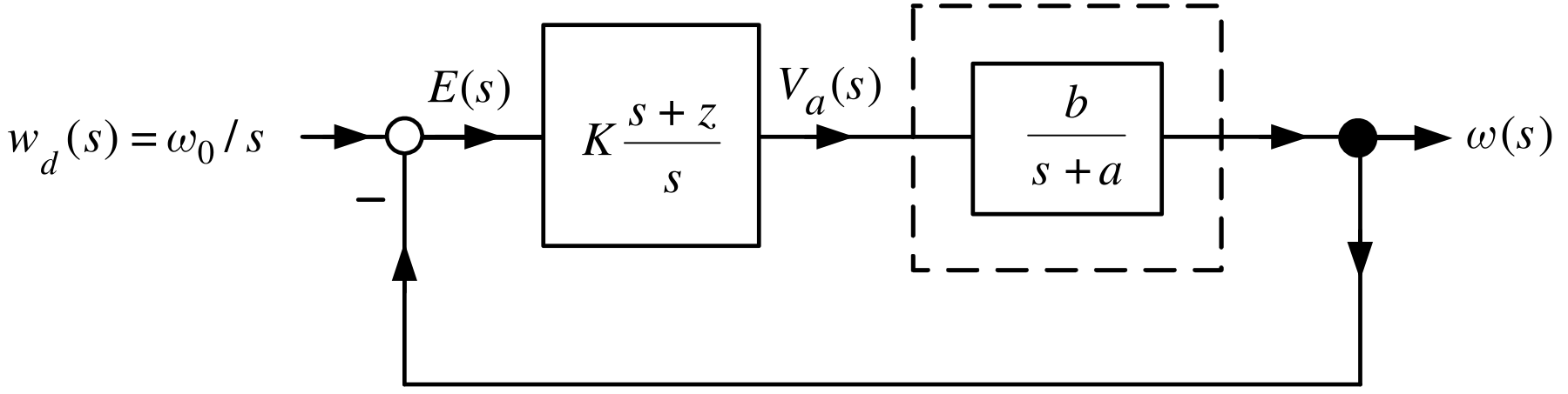
Example Speed Control of a DC Motor (continued)

\[ \!\!\!\!\!\omega(s)=\frac{\dfrac{K(s+z)}{s}\dfrac{b}{s+a}}{1+\dfrac{K(s+z)}{s}\dfrac{b}{s+a}}\frac{\omega_{0}}{s}=\frac{Kb(s+z)}{s^{2}+as+Kb(s+z)}\frac{\omega_{0}}{s}=\underset{\text{closed-loop transfer function}}{\underbrace{\frac{Kb(s+z)}{s^{2}+(a+Kb)s+Kbz}}}\text{ }\underset{\text{input}}{\underbrace{\frac{\omega_{0}}{s}}}. \]

Recall for the DC motor that \(a>0,b>0.\)
With \(K>0,z>0\) the roots of \(s^{2}+(a+Kb)s+Kbz=0\) are in the open LHP.
Thus \(s\omega(s)=\dfrac{Kb(s+z)}{s^{2}+(a+Kb)s+Kbz}\omega_{0}\) is stable.
By the FVT

\[ \omega(\infty)=\lim_{s\rightarrow0}s\omega(s)=\omega_{0}. \]

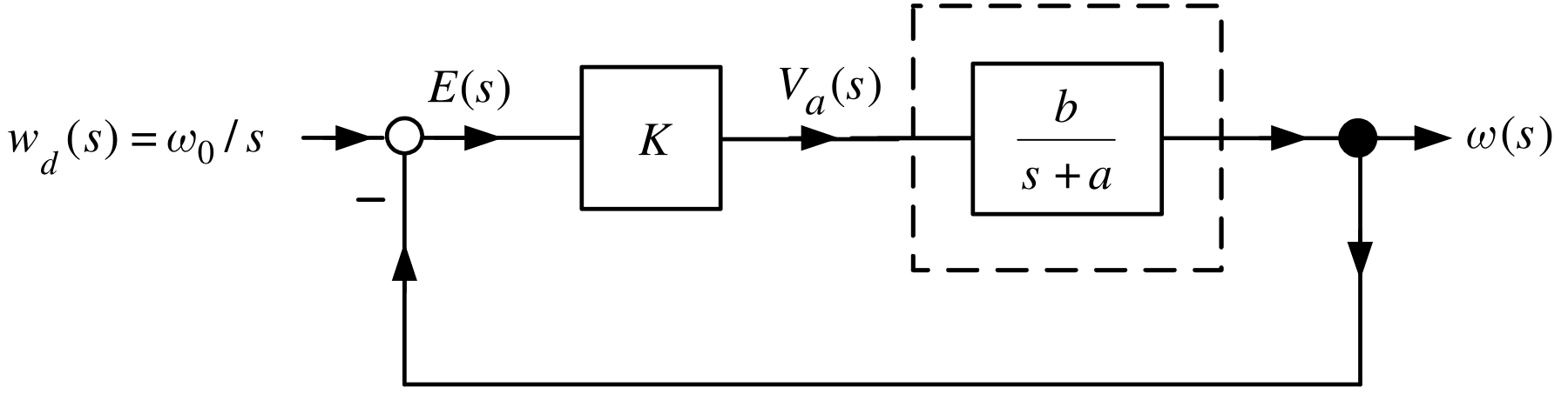
Digression Proportional Speed Control of a DC Motor

Control speed with a simple gain \(K.\)

\[ \omega(s)=\frac{K\dfrac{b}{s+a}}{1+K\dfrac{b}{s+a}}\frac{\omega_{0}}{s}=\frac{Kb}{s+a+Kb}\frac{\omega_{0}}{s}. \]

Recall for the DC motor that \(a>0,b>0.\)
With \(K>0,\) the roots of \(s+a+Kb=0\) are in the open LHP.
Thus \(s\omega(s)=\dfrac{Kb}{s+a+Kb}\omega_{0}\) is stable.
By the FVT

\[ \omega(\infty)=\lim_{s\rightarrow0}s\omega(s)=\frac{Kb}{a+Kb}\omega_{0}\neq\omega_{0}. \]

If \(K\) is large then \(\omega(\infty)\approx\omega_{0}.\)

End of Digression

Second-Order Systems with Zeros

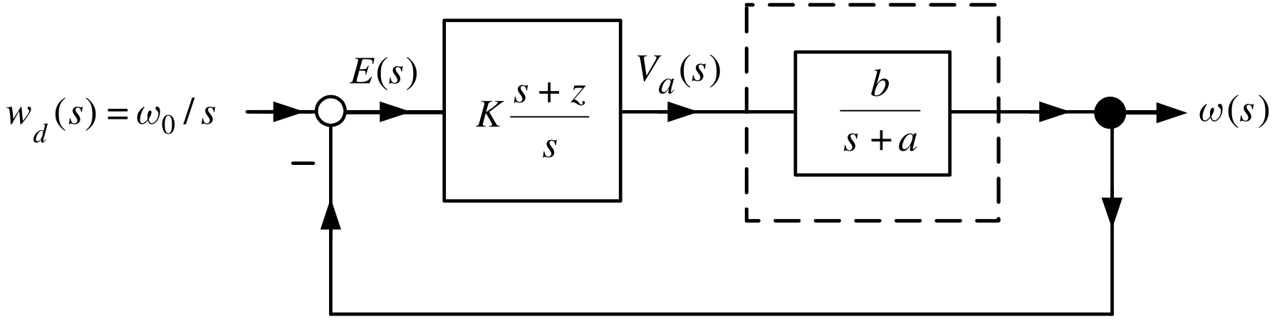
\[ \omega(s)=\frac{\dfrac{K(s+z)}{s}\dfrac{b}{s+a}}{1+\dfrac{K(s+z)}{s}\dfrac {b}{s+a}}\frac{\omega_{0}}{s}=\frac{Kb(s+z)}{s^{2}+(a+Kb)s+Kbz}\frac {\omega_{0}}{s}. \]

Let \(C(s)\triangleq\omega(s)\) and set \(\omega_{n}^{2}\triangleq Kbz,\) \(2\zeta\omega_{n}\triangleq a+Kb,\) \(\alpha\triangleq\dfrac{z}{\zeta \omega_{n}}.\)
\(Kb=\dfrac{\omega_{n}^{2}}{z}=\dfrac{\omega_{n}}{\alpha\zeta}.\)
Write

\[ C(s)=\underset{\text{closed-loop transfer function}}{\underbrace{\frac {\omega_{n}}{\alpha\zeta}\frac{s+\alpha\zeta\omega_{n}}{s^{2}+2\zeta\omega _{n}s+\omega_{n}^{2}}}}\frac{\omega_{0}}{s}. \]

What is the effect of the zero at \(s=-z=-\alpha\zeta\omega_{n}\) on the transient response?

Second-Order Systems with Zeros

Pole-Zero plot for \(0<\zeta<1.\) As the zero is in the LHP, it is a minimum phase zero.

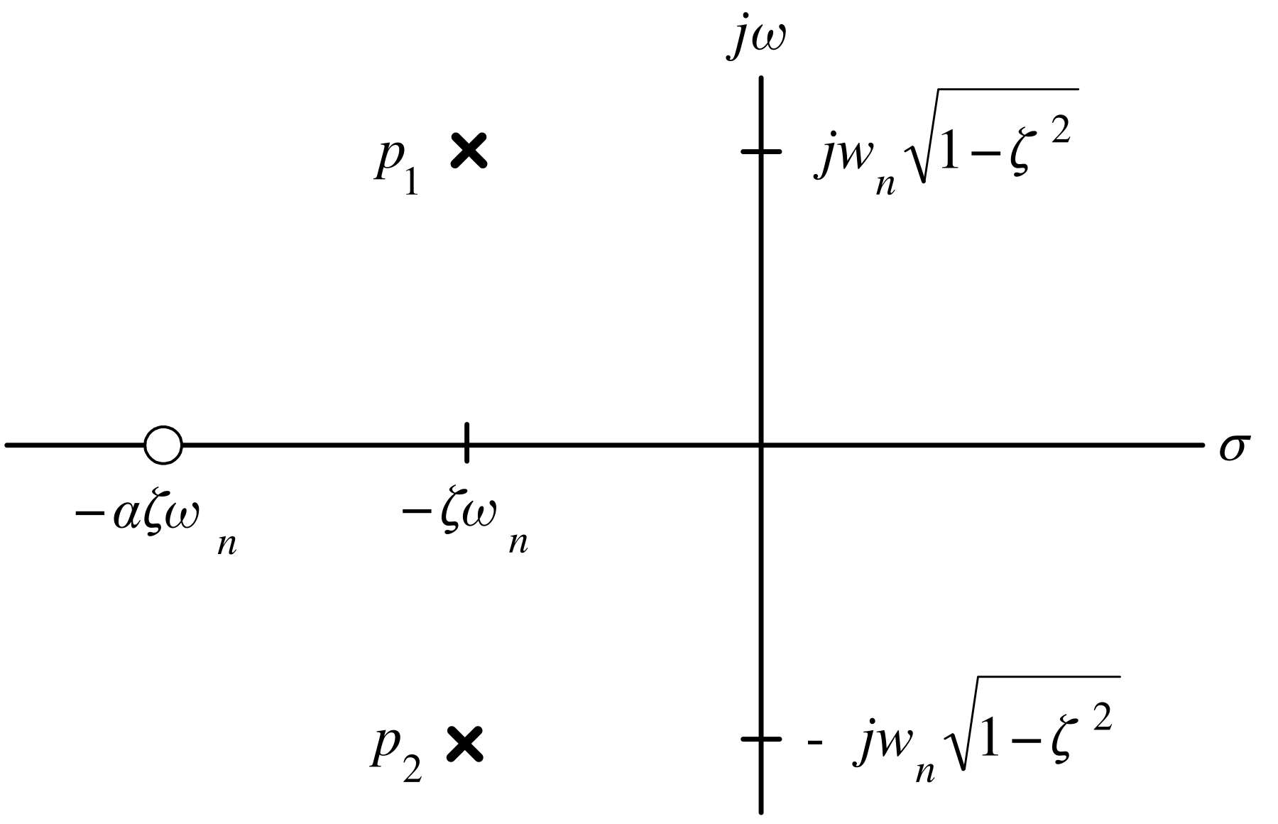
With \(\omega_{d}(s)=\dfrac{1}{s}\):

\[ \begin{aligned} C(s)=\frac{\omega_{n}}{\alpha\zeta}\frac{s+\alpha\zeta\omega_{n}}{s^{2}+2\zeta\omega_{n}s+\omega_{n}^{2}}\frac{1}{s} & =\underset{C_{1}(s)}{\underbrace{\frac{\omega_{n}^{2}}{s^{2}+2\zeta\omega_{n}s+\omega_{n}^{2}}\frac{1}{s}}}+\frac{1}{\alpha\zeta\omega_{n}}\underset{sC_{1}(s)}{\underbrace{s\frac{\omega_{n}^{2}}{s^{2}+2\zeta\omega_{n}s+\omega_{n}^{2}}\frac{1}{s}}}\\ & \rightarrow\frac{\omega_{n}^{2}}{s^{2}+2\zeta\omega_{n}s+\omega_{n}^{2}}\frac{1}{s}\text{ as }\alpha\rightarrow\infty. \end{aligned} \]

As \(\alpha\rightarrow\infty,\) \(C(s)\) reduces to \(C_{1}(s)\) which is a second-order system without a zero.

Second-Order Systems with Zeros

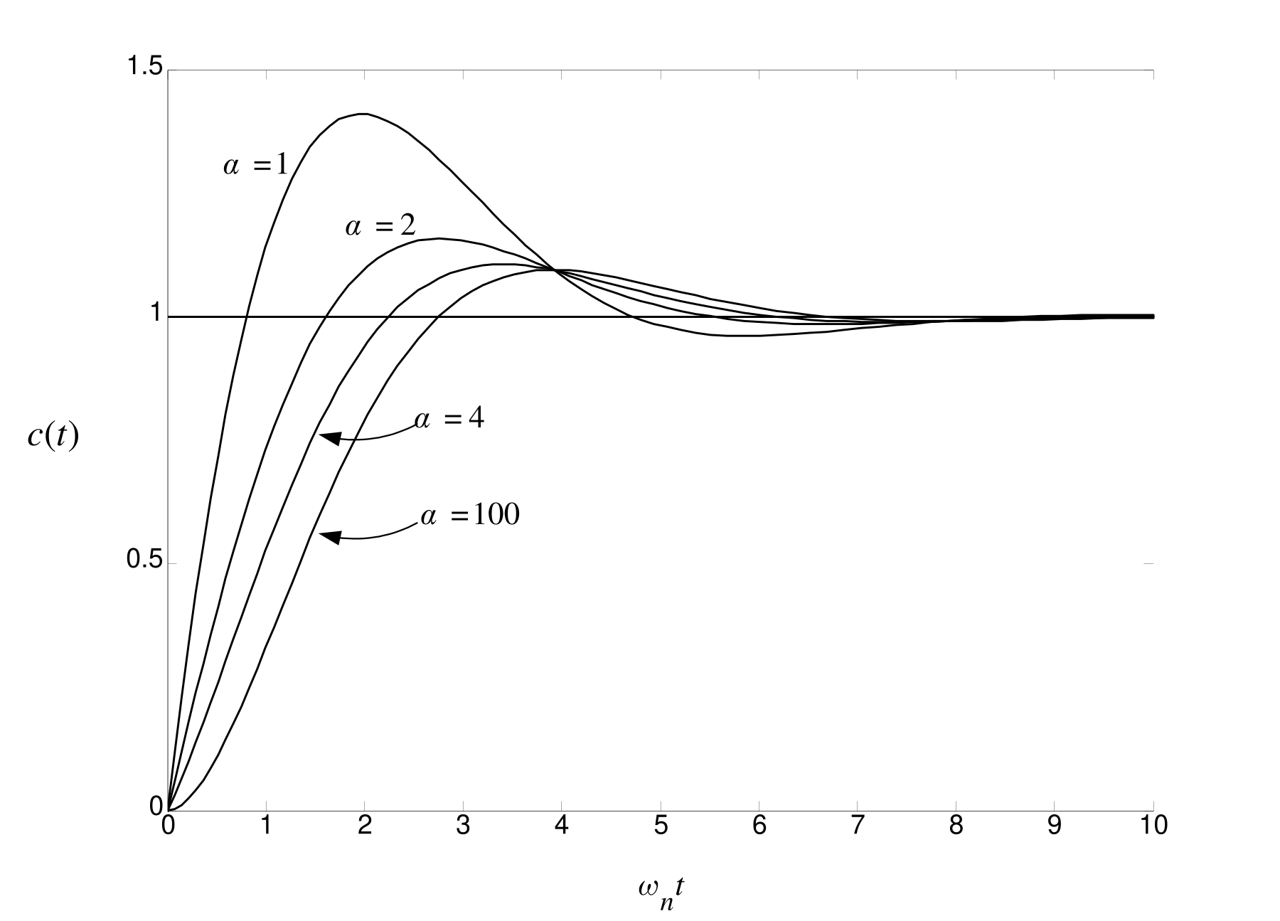
\[ c(t)=\mathcal{L}^{-1}\{C(s)\}=\mathcal{L}^{-1}\!\left\{ \frac{\omega_{n}}{\alpha\zeta}\frac{s+\alpha\zeta\omega_{n}}{s^{2}+2\zeta\omega_{n}s+\omega_{n}^{2}}\frac{1}{s}\right\} \]

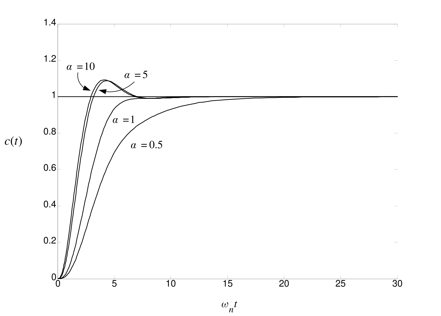
For \(\alpha>>1\) \(C(s)\) is essentially a second-order system without a zero.
Much more overshoot compared to a \(2^{nd}\) order system without a zero.

Second-Order Systems with Zeros

\[ \begin{aligned} C(s) & =\frac{\omega_{n}^{2}}{s^{2}+2\zeta\omega_{n}s+\omega_{n}^{2}}\frac {1}{s}+\frac{1}{\alpha\zeta\omega_{n}}s\frac{\omega_{n}^{2}}{s^{2}+2\zeta\omega_{n}s+\omega_{n}^{2}}\frac{1}{s}=C_{1}(s)+\frac{1}{\alpha \zeta\omega_{n}}sC_{1}(s).\\ c(t) & =c_{1}(t)+\frac{1}{\alpha\zeta\omega_{n}}\frac{dc_{1}(t)}{dt}. \end{aligned} \]

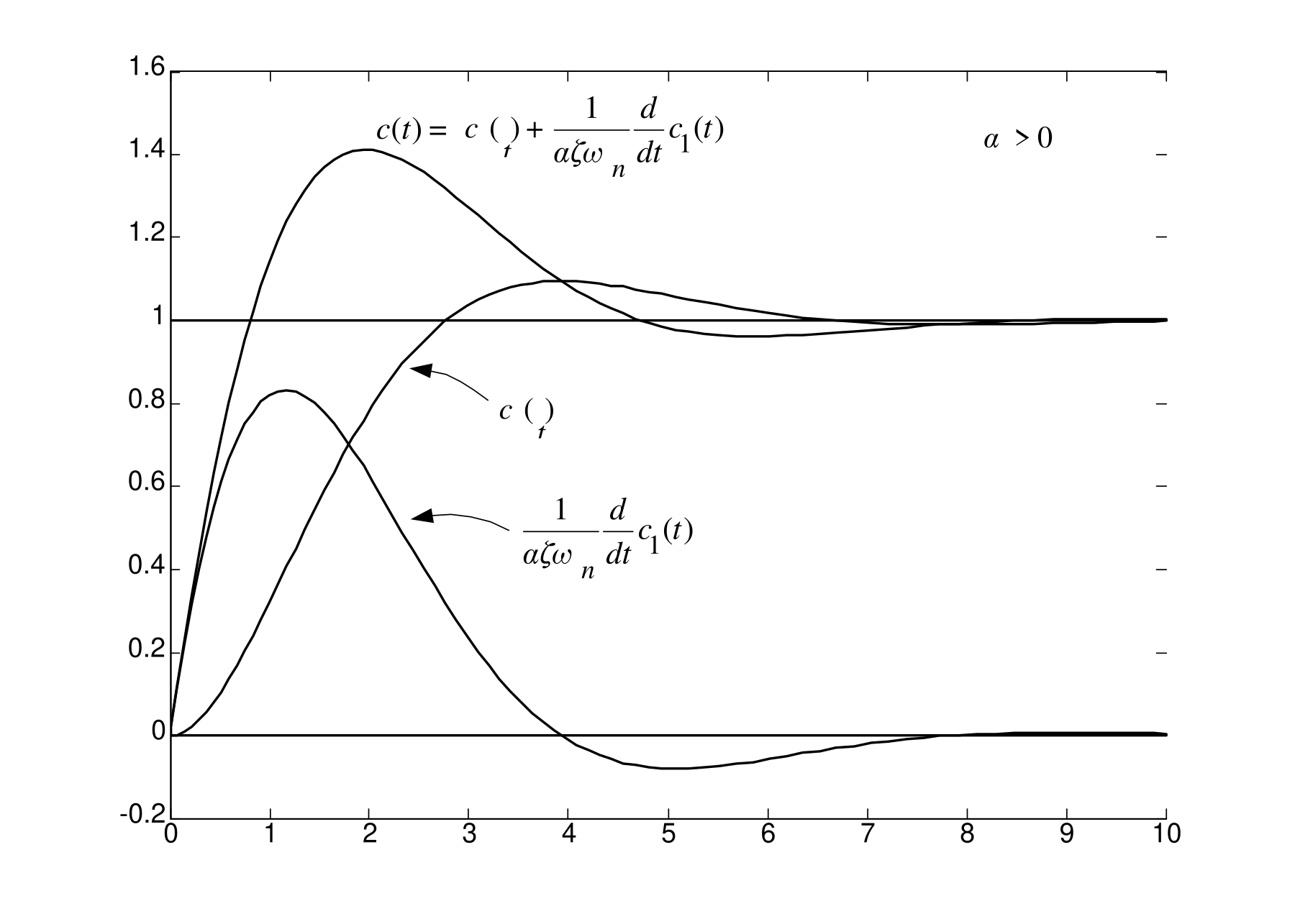
Second-Order Systems with Zeros Right Half-Plane Zero

Suppose \(\alpha<0\) so the zero \(-\alpha\zeta\omega_{n}\) is in the open RHP.
This is called a non minimum phase zero.
Pole-Zero plot for \(0<\zeta<1.\)
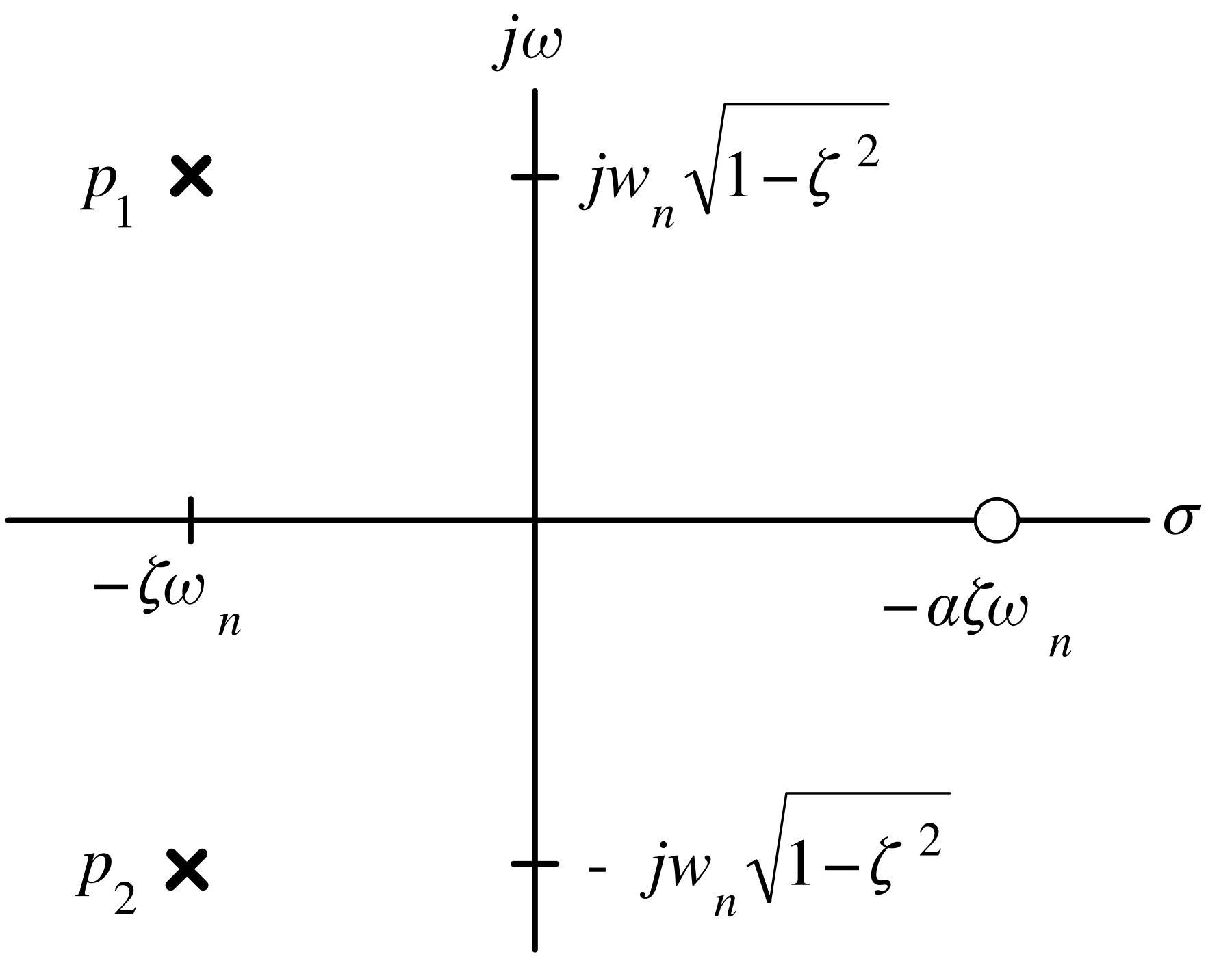
This system is still stable as the poles are in the open LHP so \(c(t)\rightarrow1\) as \(t\rightarrow\infty\).

\[ \begin{aligned} C(s)\!\! & =\!\!\frac{\omega_{n}^{2}}{s^{2}+2\zeta\omega_{n}s+\omega_{n}^{2}}\frac{1}{s}+\frac{1}{\alpha\zeta\omega_{n}}s\frac{\omega_{n}^{2}}{s^{2}+2\zeta\omega_{n}s+\omega_{n}^{2}}\frac{1}{s}=C_{1}(s)+\frac{1}{\alpha\zeta\omega_{n}}sC_{1}(s).\\ c(t)\!\! & =\!\!c_{1}(t)+\underset{<0}{\underbrace{\frac{1}{\alpha\zeta \omega_{n}}}}\frac{dc_{1}(t)}{dt}. \end{aligned} \]

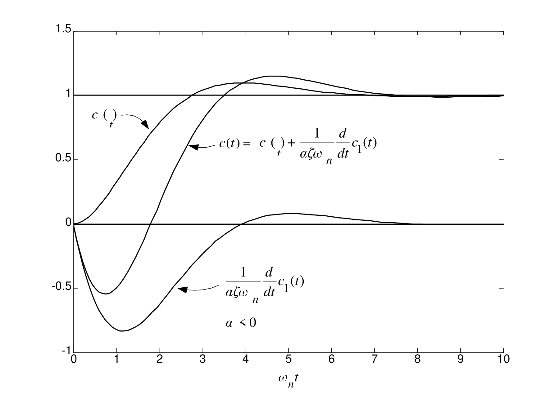
Second-Order Systems with Zeros Right Half-Plane Zero

\(c(t)\) goes negative before coming back positive - called undershoot.

Third-Order Systems

With \(0<\zeta<1\) and \(\alpha>0\) let

\[ G(s)=\frac{\alpha\zeta\omega_{n}}{s+\alpha\zeta\omega_{n}}\frac{\omega_{n}^{2}}{s^{2}+2\zeta\omega_{n}s+\omega_{n}^{2}}. \]

The poles are

\[ \begin{aligned} p_{1} & =-\zeta\omega_{n}+j\omega_{n}\sqrt{1-\zeta^{2}}\\ p_{2} & =-\zeta\omega_{n}-j\omega_{n}\sqrt{1-\zeta^{2}}\\ p_{3} & =-\alpha\zeta\omega_{n}. \end{aligned} \]

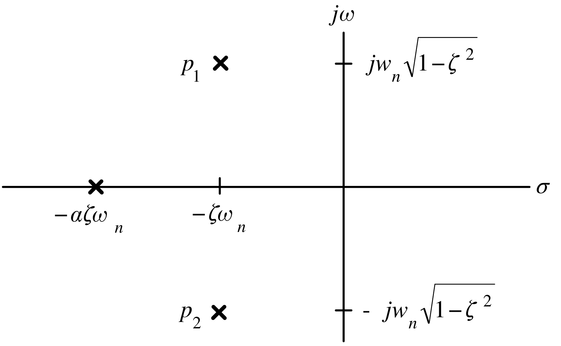
Third-Order Systems Unit Step Response

\(C(s)=G(s)\dfrac{1}{s}=\dfrac{\alpha\zeta\omega_{n}}{s+\alpha\zeta \omega_{n}}\dfrac{\omega_{n}^{2}}{s^{2}+2\zeta\omega_{n}s+\omega_{n}^{2}}\dfrac{1}{s}.\)
\(\zeta>0,\omega_{n}>0,\alpha>0\) so \(sC(s)=\dfrac{\alpha\zeta\omega_{n}}{s+\alpha\zeta\omega_{n}}\dfrac{\omega_{n}^{2}}{s^{2}+2\zeta\omega _{n}s+\omega_{n}^{2}}\) is stable.
By the FVT \(c(\infty)=\lim_{t\rightarrow\infty}c(t)=\lim_{s\rightarrow 0}sC(s)=1.\)

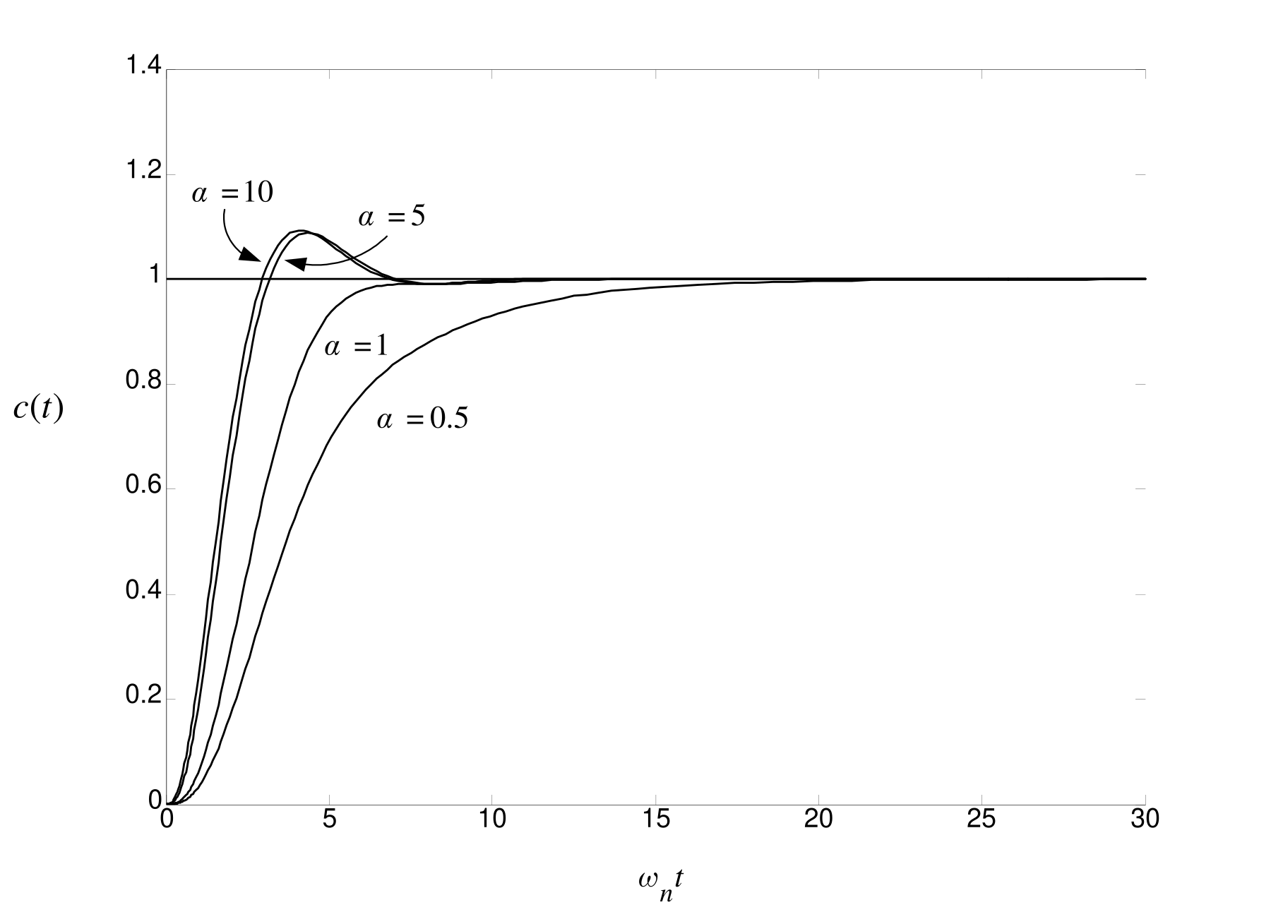
Third-Order Systems Unit Step Response

\[ C(s)=\frac{\alpha\zeta\omega_{n}}{s+\alpha\zeta\omega_{n}}\frac{\omega_{n}^{2}}{s^{2}+2\zeta\omega_{n}s+\omega_{n}^{2}}\frac{1}{s}=\frac{1}{s/\alpha\zeta\omega_{n}+1}\frac{\omega_{n}^{2}}{s^{2}+2\zeta\omega _{n}s+\omega_{n}^{2}}\frac{1}{s} \]

As \(\alpha\rightarrow\infty,\) \(C(s)\) reduces to a \(2^{nd}\) order system without a zero.
As \(\alpha\) decreases, the pole at \(-\alpha\zeta\omega_{n}\) moves closer to the \(j\omega\) axis.

\(\Longrightarrow\) The response is more sluggish as the transient dies out slower.

System Responses

Contents