Block Diagrams
System Modeling and Control · Chapter 7
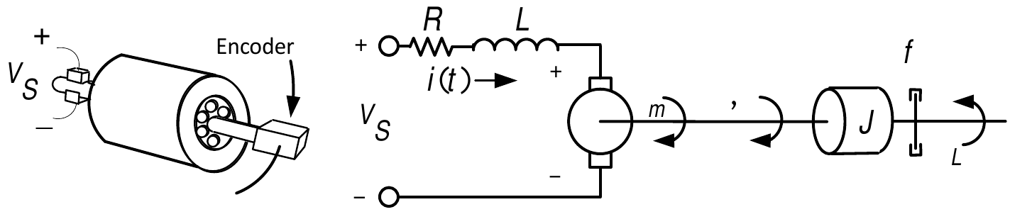
Example DC motor
\[ \begin{aligned} L\frac{di}{dt} & =-Ri-K_{b}\omega+V_{S}\\ & \\ J\frac{d\omega}{dt} & =K_{T}i-f\omega-\tau_{L}\\ & \\ \frac{d\theta}{dt} & =\omega. \end{aligned} \]
From previous slide:
\[ \begin{aligned} (sL+R)I(s) & =V_{a}(s)-K_{b}\omega(s)\\ (sJ+f)\omega(s) & =K_{T}I(s)-\tau_{L}(s)\\ s\theta(s) & =\omega(s). \end{aligned} \]
Or
\[ \begin{aligned} I(s) & =\frac{1}{sL+R}\left( V_{a}(s)-K_{b}\omega(s)\right) \\ \omega(s) & =\frac{1}{sJ+f}\left( K_{T}I(s)-\tau_{L}(s)\right) \\ \theta(s) & =\frac{1}{s}\omega(s). \end{aligned} \]
Block Diagram: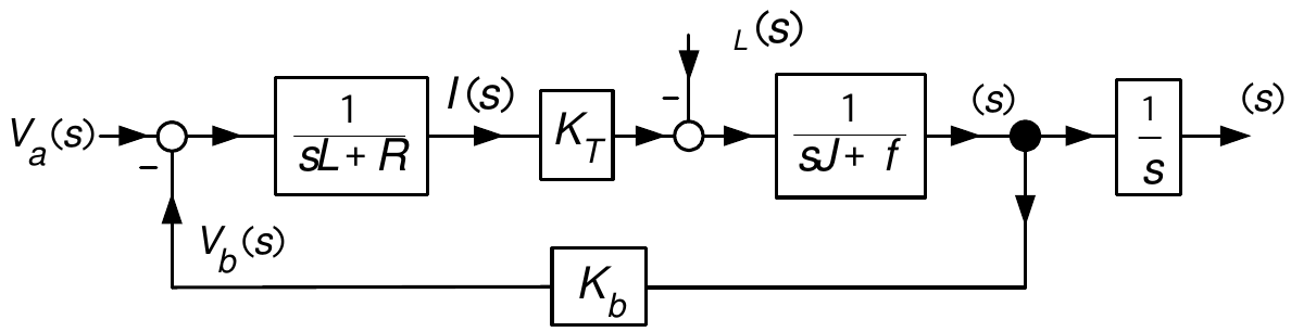
- A graphical illustration of the relationships between \(I(s),\theta (s),\omega(s),\tau_{L}(s),V_{a}(s)\)
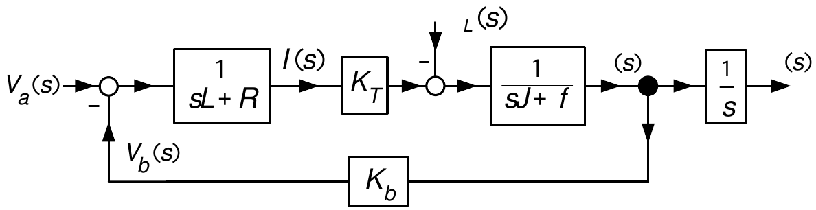
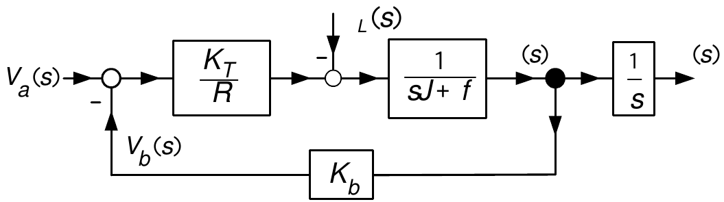
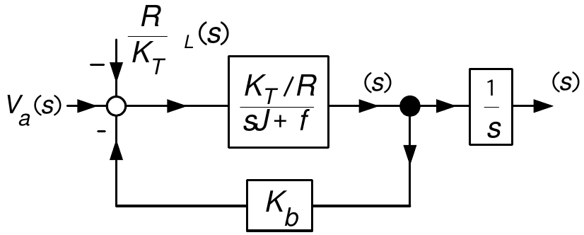
Move \(\tau_{L}(s)\) to the left side of the \(K_{T}/R\) block.
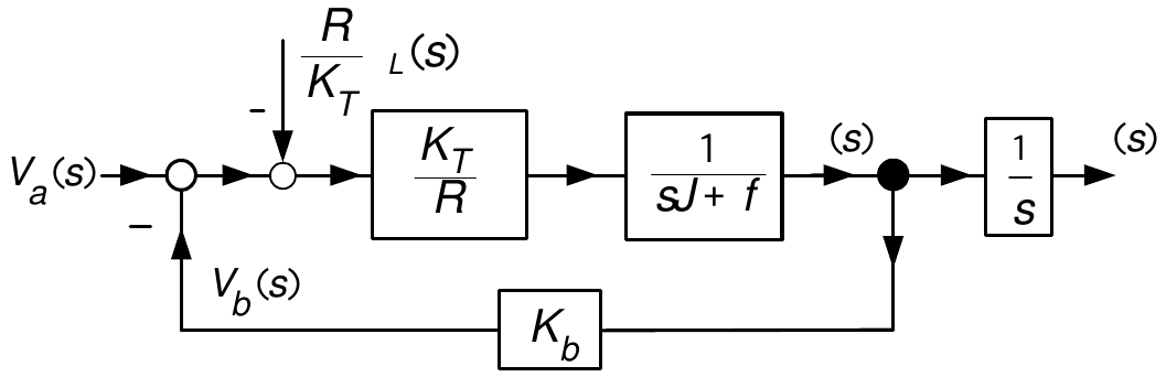
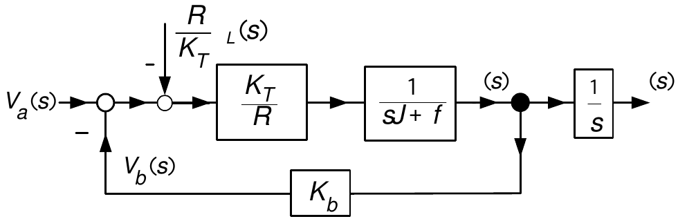
Put \(\dfrac{R}{K_{T}}\tau_{L}(s)\) into the same summing junction as \(V_{a}(s)\):
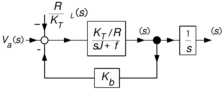
This is an equivalent block diagram to solve for \(\theta (s),\omega(s)\) in terms of \(V_{a}(s),\tau_{l}(s).\)
\(\dfrac{R}{K_{T}}\tau_{L}\) has the units of \(\frac{\text{Ohms}\times\text{Nm}}{\text{Nm/Amp}}\) = Ohms\(\times\)Amps = Volts.
The equivalent voltage \(-\dfrac{R}{K_{T}}\tau_{L}\) input to the motor has the same effect on \(\omega\) and \(\theta\) as the actual load load-torque \(\tau_{L}.\)
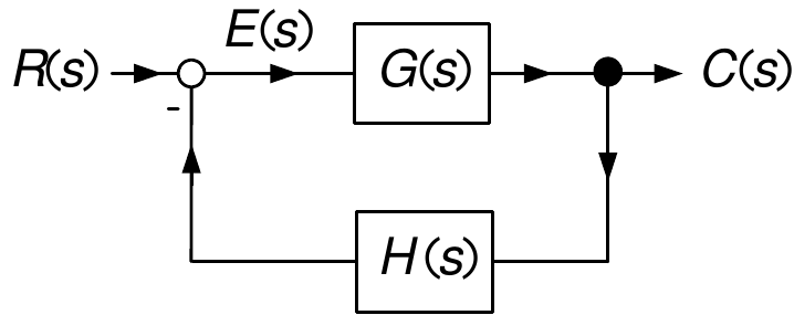
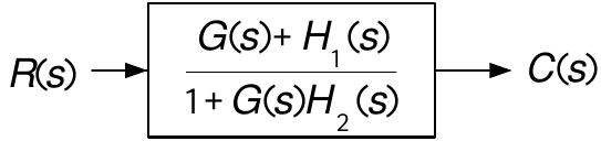
Most block diagrams are reducible to the basic block diagram:
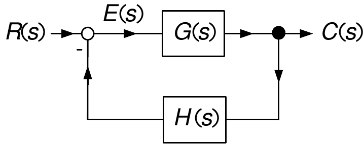
And make the identification
\[ G(s)=\frac{K_{T}/R}{sJ+f},\text{ }H(s)=K_{b},\text{ }R(s)=V_{a}(s)-\frac{R}{K_{T}}\tau_{L}(s),\text{ }C(s)=\omega(s). \]
Compute:
\[ \begin{aligned} E(s) & =R(s)-H(s)C(s)\\ & \\ C(s) & =G(s)E(s)=G(s)R(s)-G(s)H(s)C(s). \end{aligned} \]
Rearrange:
\[ (1+G(s)H(s))C(s)=G(s)R(s) \]
or
\[ C(s)=\frac{G(s)}{1+G(s)H(s)}R(s). \]
- This expression is used over and over again in the study of control systems.
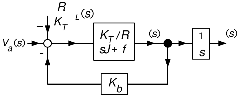
With \(G(s)=\dfrac{K_{T}/R}{sJ+f},\) \(H(s)=K_{b},\) \(R(s)=V_{a}(s)-\dfrac {R}{K_{T}}\tau_{L}(s),\) \(C(s)=\omega(s)\):
\[ \begin{aligned} \!\omega(s)\!=\!\frac{\dfrac{K_{T}/R}{sJ+f}}{1+K_{b}\dfrac{K_{T}/R}{sJ+f}}\left( \!V_{a}(s)-\frac{R}{K_{T}}\tau_{L}(s)\!\right) & =\!\frac{K_{T}/R}{sJ+f+K_{b}K_{T}/R}\!\left( \!V_{a}(s)-\frac{R}{K_{T}}\tau_{L}(s)\!\right) \\ & =\frac{\dfrac{K_{T}}{RJ}}{s+\dfrac{f+K_{b}K_{T}/R}{J}}\!\left( \!V_{a}(s)-\frac{R}{K_{T}}\tau_{L}(s)\right) \\ & =\frac{b}{s+a}\!\left( \!V_{a}(s)-K_{L}\tau_{L}(s)\!\right) \!. \end{aligned} \]
where \(a\triangleq\dfrac{f+K_{b}K_{T}/R}{J},\) \(b\triangleq\dfrac{K_{T}}{RJ},\) \(K_{L}\triangleq\dfrac{R}{K_{T}}.\)
From previous slide:
\[ \begin{aligned} \!\omega(s)\! & =\!\frac{b}{s+a}\!\left( \!V_{a}(s)-K_{L}\tau_{L}(s)\!\right) \\ & \\ a & \triangleq\dfrac{f+K_{b}K_{T}/R}{J},\text{ }b\triangleq\dfrac{K_{T}}{RJ},\text{ }K_{L}\triangleq\frac{R}{K_{T}}. \end{aligned} \]
The block diagram reduces to
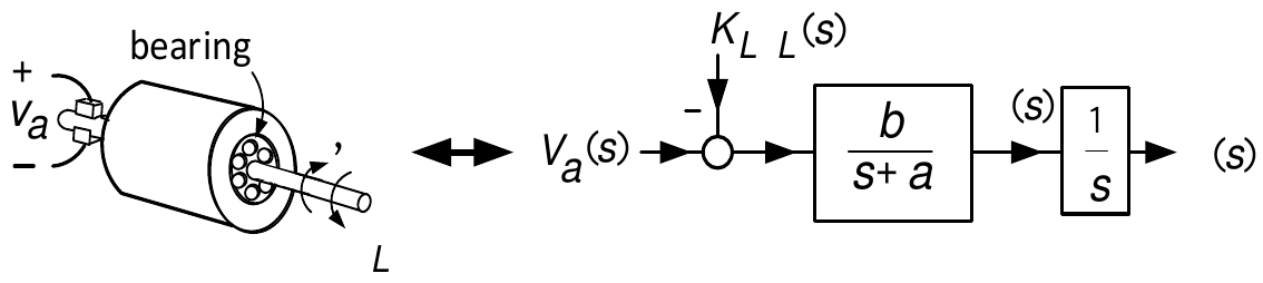
Later we describe an experiment to directly estimate the values of \(a\) and \(b\).
\(\Longrightarrow\) We don’t need to know the values of the individual motor parameters.
In practice the load torque \(\tau_{L}\) is not known.
Control problem
Use \(\theta(t)\) to compute \(v_{a}(t)\) that forces the motor to a final position \(\theta_{0}\) at time \(t_{f}\).
It must do this without knowledge of the value of \(\tau_{L}\).
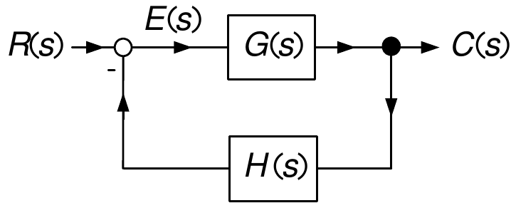
Compute the transfer function \(R(s)\) to \(E(s).\)
\[ E(s)=R(s)-H(s)C(s)=R(s)-H(s)G(s)E(s). \]
Rearrange:
\[ (1+H(s)G(s))E(s)=R(s) \]
or
\[ E(s)=\frac{1}{1+H(s)G(s)}R(s). \]
- This expression appears over and over again in the study of control systems.
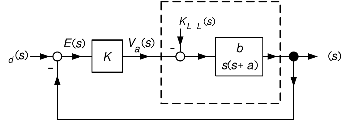
Reference input: \(\theta_{d}(s)=\dfrac{\theta_{0}}{s}\) or in the time domain \(\theta_{d}(t)=\theta_{0}u_{s}(t)\).
\(\theta_{0}\) is the desired final angular position of the motor.
\(e(t)=\theta_{0}-\theta(t)\) or in the \(s\) domain \(E(s)=\theta _{0}/s-\theta(s)\).
- This is the difference or error between the desired and actual position.
A sensor is used to measure \(\theta(t)\) and bring its value into the computer.
The value of \(\theta_{0}\) is stored in the computer.
The computer calculates \(v_{a}(t)=K(\theta_{0}-\theta(t))\).
In the \(s\) domain \(V_{a}(s)=K\!\left( \dfrac{\theta_{0}}{s}-\theta(s)\right)\).
\(v_{a}(t)=Ke(t)\) called proportional control - voltage is proportional to the error.
The value of \(v_{a}(t)\) is sent to the amplifier to apply the voltage to the motor.
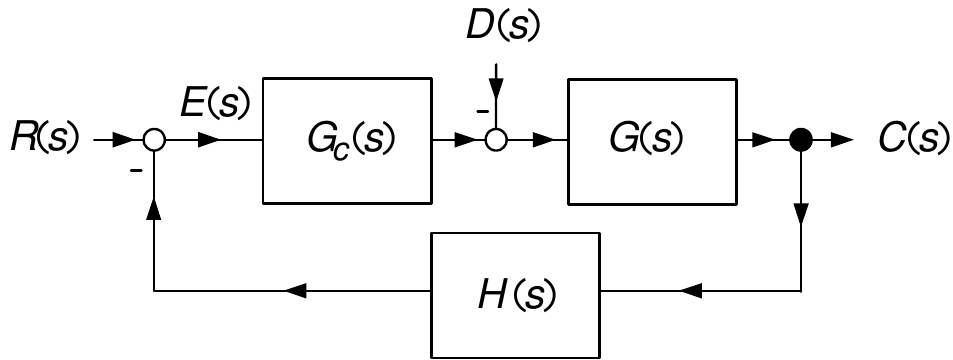
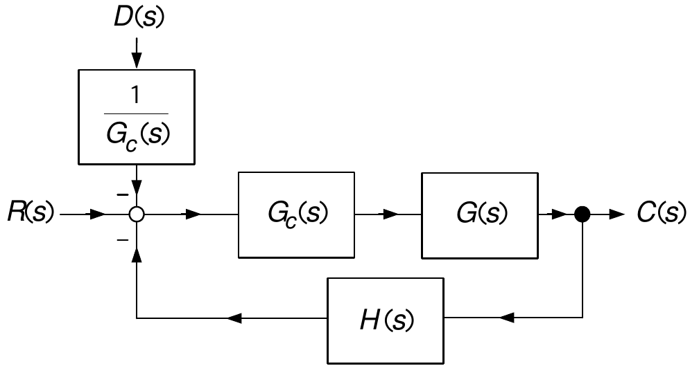
DC motor: \(G(s)=\dfrac{b}{s(s+a)},\) \(H(s)=1,\) \(G_{c}(s)=K,\) \(D(s)=K_{L}\tau_{L}(s),\) \(R(s)=\dfrac{\theta_{0}}{s}.\)
Equivalent block diagram: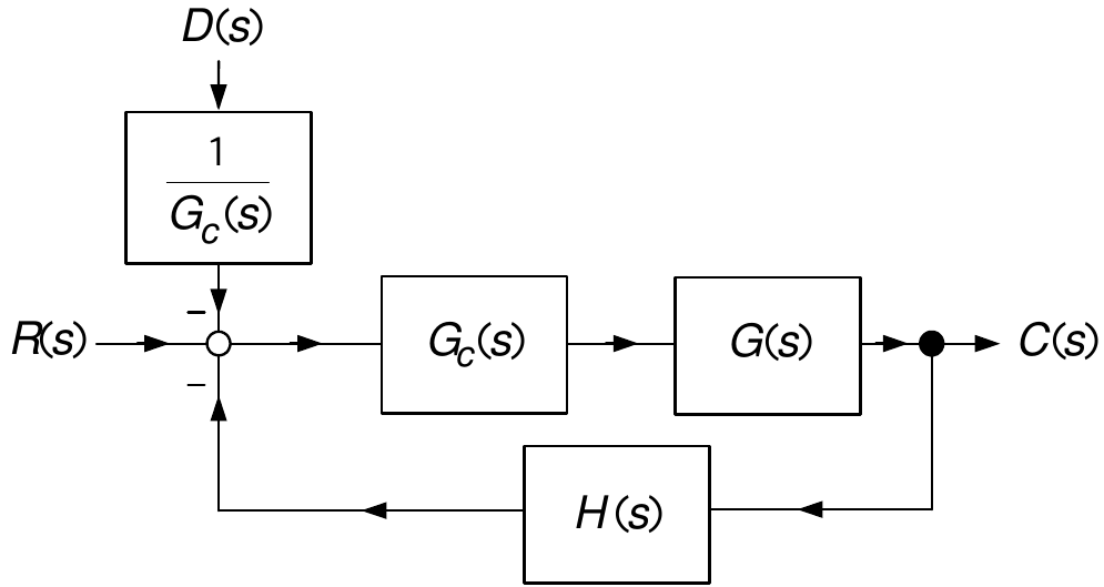
We have
\[ \begin{aligned} C(s) & =\frac{G_{c}(s)G(s)}{1+H(s)G_{c}(s)G(s)}\!\left( R(s)-\frac{1}{G_{c}(s)}D(s)\right) \\ & =\frac{G_{c}(s)G(s)}{1+H(s)G_{c}(s)G(s)}R(s)-\frac{G(s)}{1+H(s)G_{c}(s)G(s)}D(s). \end{aligned} \]
And
\[ \begin{aligned} \!\!\!\!\!E(s)=R(s)-H(s)C(s)\!\!\!\! & =\!\!\!R(s)-\!\left( \!\frac {H(s)G_{c}(s)G(s)}{1+H(s)G_{c}(s)G(s)}R(s)-\frac{H(s)G(s)}{1+H(s)G_{c}(s)G(s)}D(s)\!\!\right) \\ \!\!\!\!\! & =\!\!\!\frac{1}{1+H(s)G_{c}(s)G(s)}R(s)+\frac{H(s)G(s)}{1+H(s)G_{c}(s)G(s)}D(s). \end{aligned} \]
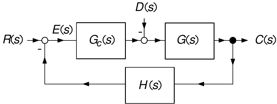
Most often we use unity feedback, i.e., \(H(s)=1\). Then
\[ \begin{aligned} C(s) & =\frac{G_{c}(s)G(s)}{1+G_{c}(s)G(s)}R(s)-\frac{G(s)}{1+G_{c}(s)G(s)}D(s)\\ & \\ E(s) & =\frac{1}{1+G_{c}(s)G(s)}R(s)+\frac{G(s)}{1+G_{c}(s)G(s)}D(s). \end{aligned} \]
- We will make extensive use of these in the design of the feedback controller \(G_{c}(s)\).
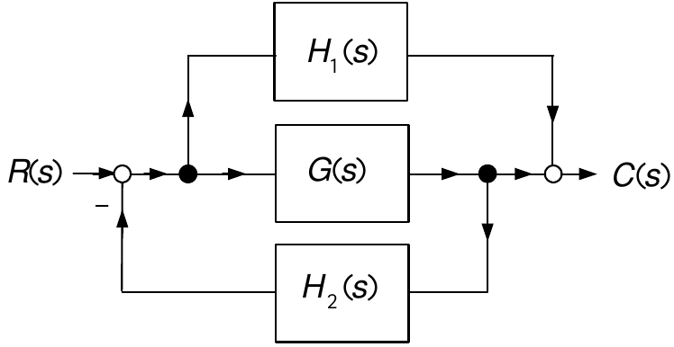
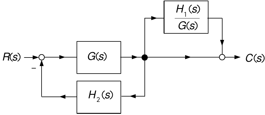

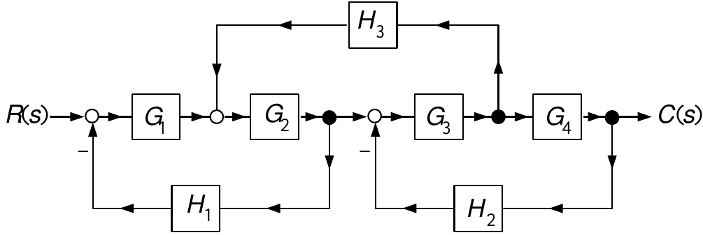
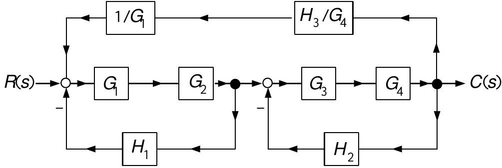
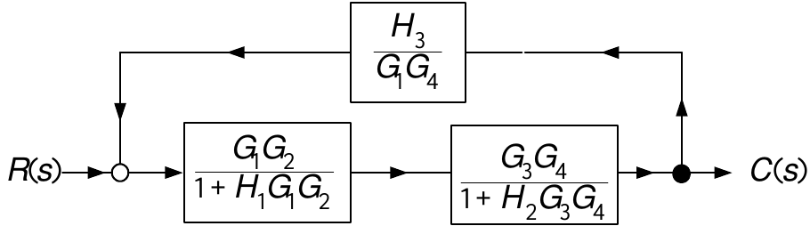
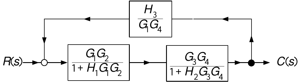
- Note that a minus sign is missing in the feedback path!
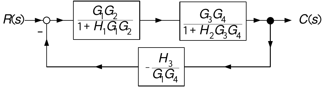
Then
\[ C(s)=\frac{\dfrac{G_{1}G_{2}}{1+H_{1}G_{1}G_{2}}\dfrac{G_{3}G_{4}}{1+H_{2}G_{3}G_{4}}}{1-\dfrac{H_{3}}{G_{1}G_{2}}\dfrac{G_{1}G_{2}}{1+H_{1}G_{1}G_{2}}\dfrac{G_{3}G_{4}}{1+H_{2}G_{3}G_{4}}}R(s). \]
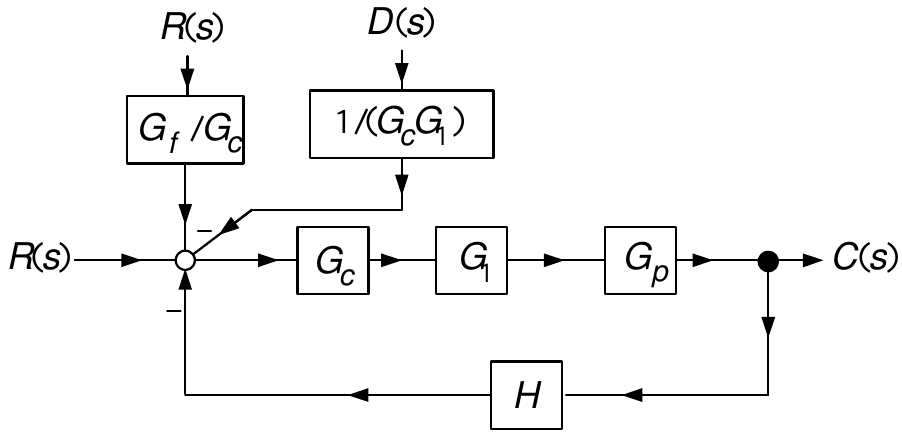
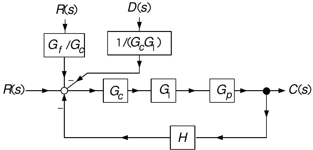
Then
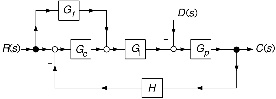
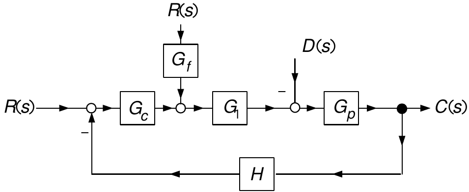
\[ \begin{aligned} C(s) & =\frac{G_{c}G_{1}G_{p}}{1+HG_{c}G_{1}G_{p}}\left( R(s)+\frac{G_{f}}{G_{c}}R(s)-\frac{1}{G_{c}G_{1}}D(s)\right) \\ & \\ & \\ & =\frac{G_{1}G_{p}(G_{c}+G_{f})}{1+HG_{c}G_{1}G_{p}}R(s)-\frac{G_{p}}{1+HG_{c}G_{1}G_{p}}D(s) \end{aligned} \]
The input to the motor is the voltage \(v_{a}\).
The motor torque is \(K_{T}i.\)
Use feedback to make current (and therefore torque) the input.
Recall
\[ I(s)=\frac{-K_{b}\omega(s)+V_{a}(s)}{sL+R},\text{ }\omega(s)=\frac {K_{T}I(s)-\tau_{L}(s)}{sJ+f},\text{ }\theta(s)=\frac{1}{s}\omega(s). \]
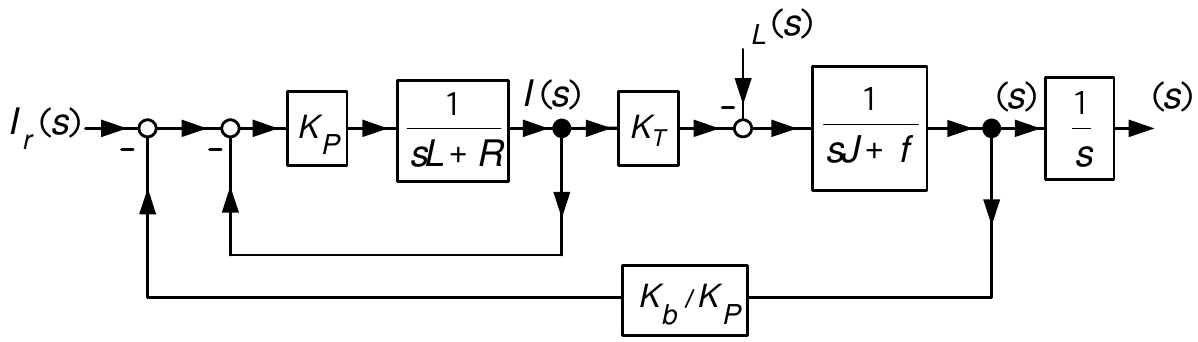
Block diagram with current feedback: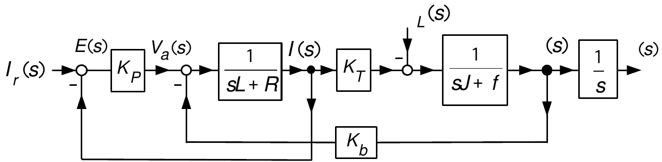
\(I_{r}(s)\) is the LT of the reference (desired) motor current.
\(I(s)\) is the LT of the motor current.
\(K_{P}>0\) is a proportional gain.
We do not set \(L=0.\)
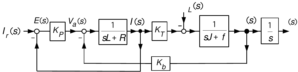
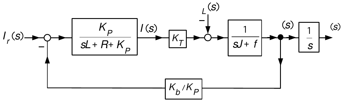
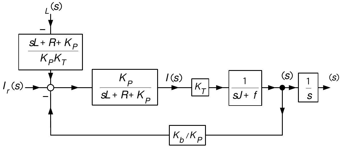
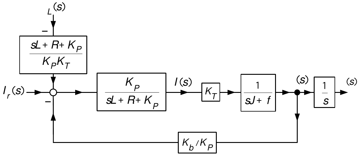
\[ \begin{aligned} \omega(s)\! & =\!\!\frac{\dfrac{K_{p}}{sL+R+K_{p}}\dfrac{K_{T}}{sJ+f}}{1+\dfrac{K_{b}}{K_{p}}\dfrac{K_{p}}{sL+R+K_{p}}\dfrac{K_{T}}{sJ+f}}\!\left( \!I_{r}(s)-\frac{1}{\dfrac{K_{p}K_{T}}{sL+R+K_{p}}}\tau_{L}(s)\!\!\right) \\ & \\ \!\! & =\!\!\frac{\overset{\rightarrow1\text{ as }K_{p}\rightarrow \infty}{\overbrace{\dfrac{1}{(sL+R)/K_{p}+1}}}\dfrac{K_{T}}{sJ+f}}{1+\underset{\rightarrow0}{\underbrace{\dfrac{K_{b}}{K_{p}}}}\underset{\rightarrow1\text{ as }K_{p}\rightarrow\infty}{\underbrace{\dfrac {1}{(sL+R)/K_{p}+1}}}\dfrac{K_{T}}{sJ+f}}\!\left( \!I_{r}(s)-\frac {1}{\underset{\rightarrow1\text{ as }K_{p}\rightarrow\infty }{\underbrace{\dfrac{1}{(sL+R)/K_{p}+1}}}K_{T}}\tau_{L}(s)\!\!\right) \end{aligned} \]
- By letting \(K_{p}\rightarrow\infty\) we obtain \(\dfrac{1}{(sL+R)/K_{p}+1}\rightarrow1\) and \(\dfrac{K_{b}}{K_{p}}\rightarrow0.\)
\[ \omega(s)=\frac{\dfrac{K_{T}}{sJ+f}}{1}\!\left( I_{r}(s)-\frac{1}{K_{T}}\tau_{L}(s)\right) =\dfrac{K_{T}}{sJ+f}\left( I_{r}(s)-\frac{1}{K_{T}}\tau_{L}(s)\right) . \]
Block diagram is simply
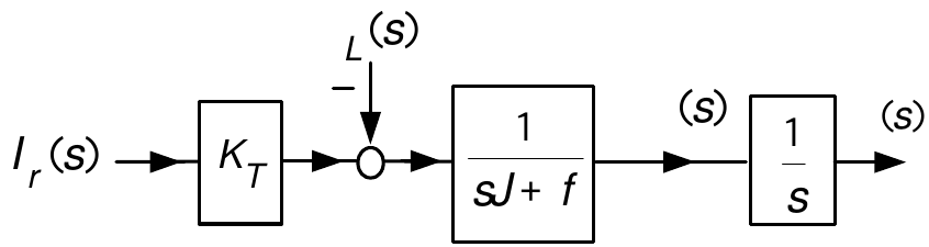
If the gain \(K_{P}\) is large enough, \(i(t)\) is forced to track \(i_{r}(t).\)
- We can then assume that \(i_{r}\) is essentially equal to \(i\).
However, \(K_{P}\) cannot be arbitrarily large.
\(v_{a}(t)=K_{P}(i_{r}(t)-i(t))\) which for large \(K_{P}\) can make \(v_{a}\) greater than \(V_{\text{max}}\).
With a good current controller, \(v_{a}(t)\) automatically adjusts to force \(i(t)\rightarrow i_{r}(t)\).
We can now design the feedback controller with \(i_{r}(t)\) as the input.
