The Physics of the DC Motor

System Modeling and Control · Chapter 6

John N. Chiasson and Aykut C. Satici

Magnetic Force
Faraday’s Law
Dynamic Equations of the DC Motor
Optical Encoder Model

Magnetic Force

Magnetic fields produce forces on wires carrying a current.
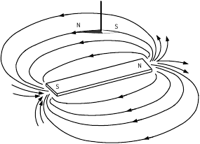
The direction of \(\vec{\mathbf B}\) at any point is the direction a compass needle points.

The magnetic force is proportional to the wire length \(\ell\) and current \(i\): \(F_{\text{magnetic}}\propto \ell i\).

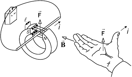
The field magnitude is \(B=\lvert\vec{\mathbf B}\rvert\triangleq F_{\text{magnetic}}/(\ell i)\).

Magnetic Force Law

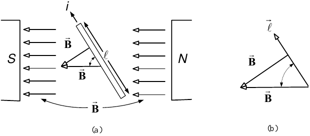
The magnetic force is proportional to the current \(i\), wire length \(\ell\), field strength \(B=\lvert\vec{\mathbf B}\rvert\), and the sine of the angle between \(\vec{\mathbf B}\) and the wire.

For \(\vec{\ell}\), the magnitude \(\ell=\lvert\vec{\ell}\rvert\) is the length of wire in the magnetic field, and its direction is the direction of positive current.

\[ \begin{aligned} \vec{\mathbf F}_{\text{magnetic}} &= i\vec{\ell}\times\vec{\mathbf B},\\ F_{\text{magnetic}} &= i\ell B\sin\theta=i\ell B_{\perp}. \end{aligned} \]

Example Linear DC Machine

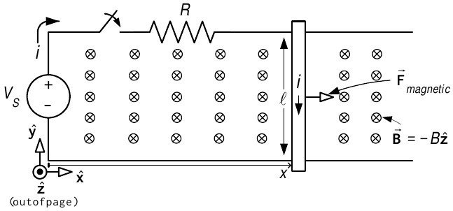
\[ \vec{\mathbf B}=-B\hat{\mathbf z},\quad B>0, \qquad \vec{\ell}=-\ell\hat{\mathbf y}. \]

\[ \vec{\mathbf F}_{\text{magnetic}} =i\vec{\ell}\times\vec{\mathbf B} =i(-\ell\hat{\mathbf y})\times(-B\hat{\mathbf z}) =i\ell B\hat{\mathbf x}. \]

\(f\) is the coefficient of viscous sliding friction.
\(m_{\ell}\) is the mass of the bar.
Equation of motion: \[i\ell B-f\frac{dx}{dt}=m_{\ell}\frac{d^{2}x}{dt^{2}}.\]

Example Single-Loop Motor

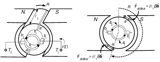
A soft-iron cylindrical core is placed inside a hollowed-out permanent magnet.
The magnetic field tends to be perpendicular to the surface of magnetic materials.
The cylindrical shape makes \(\vec{\mathbf B}\) radially directed in the air gap.

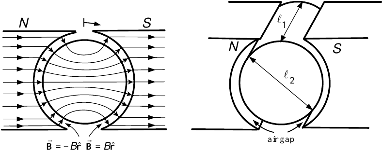
For \(B>0\),

\[ \vec{\mathbf B}= \begin{cases} +B\hat{\mathbf r}, & 0<\theta<\pi,\\ -B\hat{\mathbf r}, & \pi<\theta<2\pi. \end{cases} \]

Rotor Loop and Slip Rings

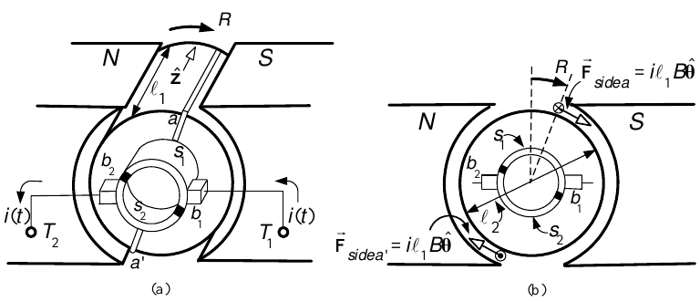
\(\hat{\mathbf r}\), \(\hat{\boldsymbol\theta}\), and \(\hat{\mathbf z}\) denote the cylindrical-coordinate unit vectors.
\(\hat{\mathbf z}\) points along the rotor axis into the page.
\(\hat{\boldsymbol\theta}\) points in the direction of increasing \(\theta\); \(\hat{\mathbf r}\) points in the direction of increasing \(r\).

Single-Loop Motor: Torque

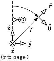
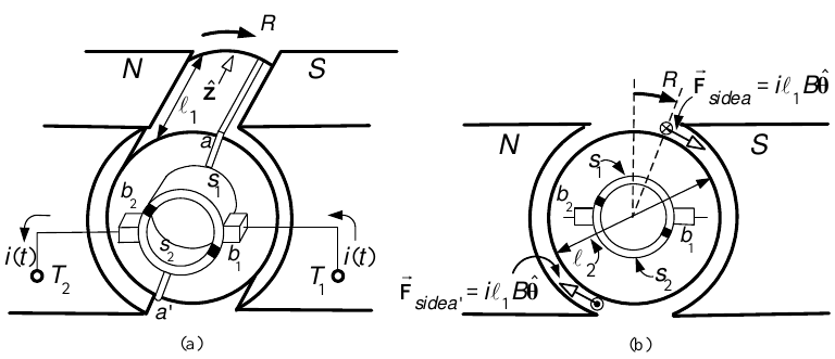
For \(i>0\), current in side \(a\) goes into the page, so \(\vec{\ell}=\ell_{1}\hat{\mathbf z}\).

\[ \vec{\mathbf F}_{a} =i(\ell_{1}\hat{\mathbf z})\times(B\hat{\mathbf r}) =i\ell_{1}B\hat{\boldsymbol\theta}. \]

\[ \begin{aligned} \vec{\boldsymbol\tau}_{a} &=\frac{\ell_{2}}{2}\hat{\mathbf r}\times\vec{\mathbf F}_{a}\\ &=\frac{\ell_{2}}{2}i\ell_{1}B (\hat{\mathbf r}\times\hat{\boldsymbol\theta}) =\frac{\ell_{2}}{2}i\ell_{1}B\hat{\mathbf z}. \end{aligned} \]

Single-Loop Motor: Total Torque

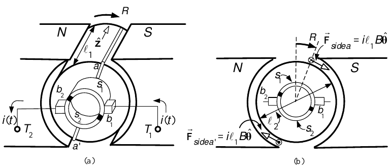
On side \(a'\),

\[ \vec{\mathbf F}_{a'} =i(-\ell_{1}\hat{\mathbf z})\times(-B\hat{\mathbf r}) =i\ell_{1}B\hat{\boldsymbol\theta}, \]

\[ \vec{\boldsymbol\tau}_{a'} =\frac{\ell_{2}}{2}\hat{\mathbf r}\times\vec{\mathbf F}_{a'} =\frac{\ell_{2}}{2}i\ell_{1}B\hat{\mathbf z}. \]

Thus \[ \vec{\boldsymbol\tau}_{m}=\ell_{1}\ell_{2}Bi\hat{\mathbf z}, \qquad \tau_{m}=K_{T}i, \qquad K_{T}\triangleq\ell_{1}\ell_{2}B. \]

Current Commutation

To obtain positive torque \(\tau_{m}=K_{T}i>0\):

Current under the south pole must go into the page.
Current under the north pole must come out of the page.
Every half-turn, the direction of current in the loop must reverse.

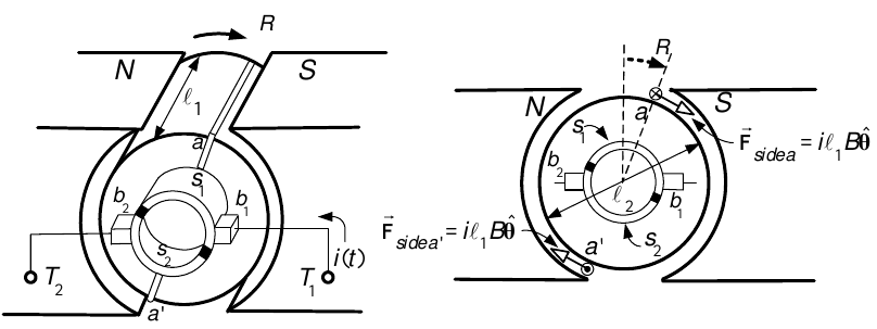
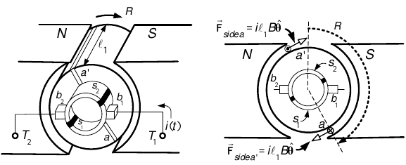
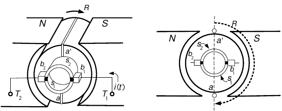
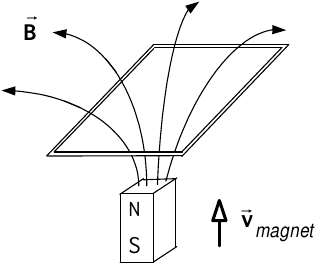
Current Commutation Through One Rotation

Faraday’s Law

A changing magnetic flux in a loop produces an induced voltage, or electromotive force (emf), denoted by \(\xi\):

\[ \xi=-\frac{d\phi}{dt}, \qquad \phi=\int_{S}\vec{\mathbf B}\cdot d\vec{\mathbf S}. \]

Here \(S\) is any surface whose boundary is the loop.

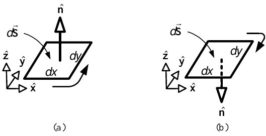
The Surface-Element Vector \(d\vec{\mathbf S}\)

The surface-element vector may be oriented in either normal direction:

\[ d\vec{\mathbf S}=dx\,dy\,\hat{\mathbf z} \qquad\text{or}\qquad d\vec{\mathbf S}=-dx\,dy\,\hat{\mathbf z}. \]

The corresponding positive direction around the boundary follows the right-hand rule.

Connecting two surface elements:

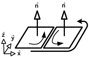
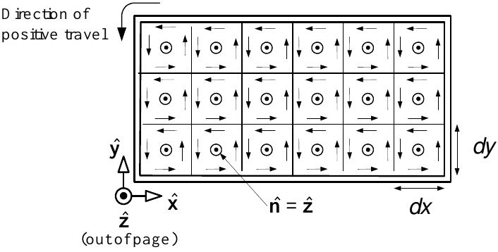
Net Direction Around a Surface Boundary

The normal is \(\hat{\mathbf n}=\hat{\mathbf z}\).
\(d\vec{\mathbf S}=dx\,dy\,\hat{\mathbf n}=dx\,dy\,\hat{\mathbf z}\).
\(\odot\) denotes a normal directed out of the page.
Positive travel around the boundary is counterclockwise.

Interpreting the Sign of \(\xi\)

\[ \xi=-\frac{d\phi}{dt}, \qquad \phi=\int_{S}\vec{\mathbf B}\cdot d\vec{\mathbf S}. \]

If \(\xi>0\), the induced emf drives current in the positive direction of travel.
If \(\xi<0\), the induced emf drives current in the opposite direction.

Simple examples make the sign convention concrete.

Example Linear DC Machine

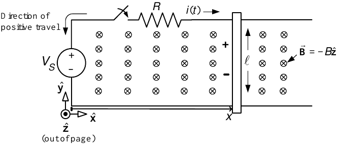
Let \(\vec{\mathbf B}=-B\hat{\mathbf z}\), \(B>0\), and choose \(d\vec{\mathbf S}=dx\,dy\,\hat{\mathbf z}\). Then

\[ \phi=\int_{0}^{\ell}\int_{0}^{x} (-B\hat{\mathbf z})\cdot(dx\,dy\,\hat{\mathbf z})=-B\ell x. \]

Therefore \[ \xi=-\frac{d\phi}{dt}=B\ell\frac{dx}{dt}=B\ell v. \]

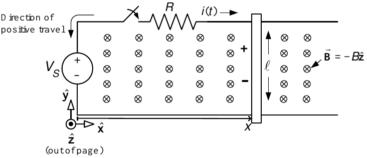
Example Linear DC Machine (continued)

We found \(\xi=B\ell v\).

The magnetic force is \(\vec{\mathbf F}_{\text{magnetic}}=i\ell B\hat{\mathbf x}\), so \(v=dx/dt>0\).
The induced voltage \(\xi>0\) opposes the source voltage \(V_{S}\).

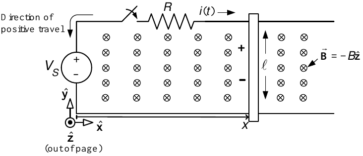
Energy Conversion in a Linear DC Machine

\(F_{\text{magnetic}}=i\ell B\).
Mechanical power produced: \(F_{\text{magnetic}}v=i\ell Bv\).
The back emf \(\xi=B\ell v\) opposes current \(i\).
Electrical power absorbed by the back emf: \(-i\xi=-iB\ell v\).

The electrical power absorbed reappears as mechanical power: \[ -i\xi+F_{\text{magnetic}}v=-iB\ell v+i\ell Bv=0. \]

Linear DC Machine: Equations of Motion

Take circuit self-inductance as zero. Let \(m_{\ell}\) be the bar mass and \(f\) the viscous-friction coefficient.

\[ \begin{aligned} V_{S}-B\ell v &= Ri,\\ m_{\ell}\frac{dv}{dt} &= i\ell B-fv. \end{aligned} \]

Eliminating \(i\) gives \[ m_{\ell}\frac{d^{2}x}{dt^{2}} =-\left(\frac{B^{2}\ell^{2}}{R}+f\right)\frac{dx}{dt} +\frac{\ell B}{R}V_{S}, \]

or \[ \frac{dx}{dt}=v, \qquad \frac{dv}{dt} =-\left(\frac{B^{2}\ell^{2}}{m_{\ell}R}+\frac{f}{m_{\ell}}\right)v +\frac{\ell B}{m_{\ell}R}V_{S}. \]

Example EMF in the Single-Loop Motor

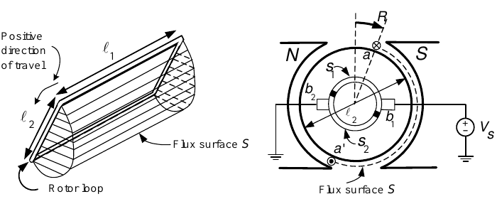
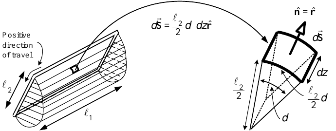
On the cylindrical surface, \(d\vec{\mathbf S}=(\ell_{2}/2)d\theta\,dz\,\hat{\mathbf r}\).
On the two half-disk ends, \(\vec{\mathbf B}\cdot d\vec{\mathbf S}=0\).

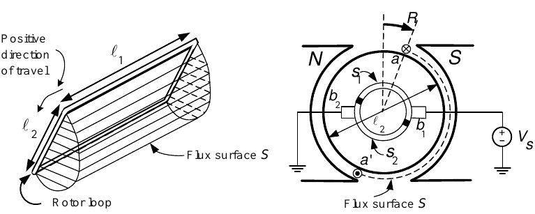
Example EMF in the Single-Loop Motor (continued)

For \(0<\theta_{R}<\pi\),

\[ \begin{aligned} \phi(\theta_{R}) &=\int_{0}^{\ell_{1}}\int_{\theta_{R}}^{\pi} B\frac{\ell_{2}}{2}\,d\theta\,dz +\int_{0}^{\ell_{1}}\int_{\pi}^{\pi+\theta_{R}} (-B)\frac{\ell_{2}}{2}\,d\theta\,dz\\ &=\frac{\ell_{1}\ell_{2}B}{2}(\pi-\theta_{R}) -\frac{\ell_{1}\ell_{2}B}{2}\theta_{R}\\ &=-\ell_{1}\ell_{2}B\left(\theta_{R}-\frac{\pi}{2}\right). \end{aligned} \]

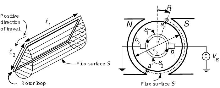
Example EMF in the Single-Loop Motor (continued)

For \(0<\theta_{R}<\pi\), \[ \phi(\theta_{R})=-\ell_{1}\ell_{2}B \left(\theta_{R}-\frac{\pi}{2}\right). \]

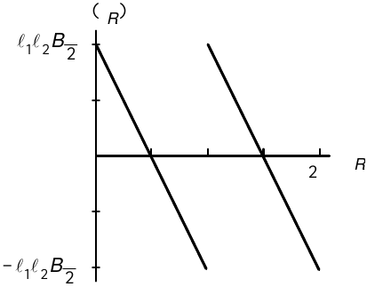
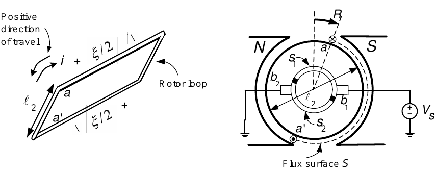
Example EMF in the Single-Loop Motor (continued)

\[ \phi(\theta_{R})=-\ell_{1}\ell_{2}B \left(\theta_{R}-\frac{\pi}{2}\right), \qquad 0<\theta_{R}<\pi. \]

Faraday’s law gives \[ \xi=-\frac{d\phi}{dt} =(\ell_{1}\ell_{2}B)\frac{d\theta_{R}}{dt} =K_{b}\omega_{R}, \qquad K_{b}\triangleq\ell_{1}\ell_{2}B. \]

For \(\omega_{R}>0\), \(\xi>0\) and the back emf opposes \(V_{S}\).

Example EMF in the Single-Loop Motor (continued)

Energy Conversion in the Single-Loop Motor

Mechanical power produced:

\[ \tau_{m}\omega_{R} =K_{T}i\omega_{R} =\ell_{1}\ell_{2}Bi\omega_{R}. \]

Electrical power absorbed by the back emf:

\[ -\xi i =-K_{b}\omega_{R}i =-\ell_{1}\ell_{2}B\omega_{R}i. \]

The electrical power absorbed reappears as mechanical power:

\[ -\xi i+\tau_{m}\omega_{R}=0. \]

Therefore energy conservation requires

\[ K_{T}=K_{b}. \]

Self-Inductance \(L\): Rotor Current Produces Flux

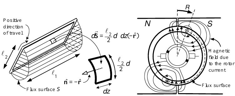
The magnetic field on the flux surface due to armature current has the form \[ \vec{\mathbf B}(r_{R},\theta-\theta_{R},i) =-iK(r_{R},\theta-\theta_{R})\hat{\mathbf r}, \] where \[ K>0\quad\text{for }0\leq\theta-\theta_{R}\leq\pi, \qquad K<0\quad\text{for }\pi\leq\theta-\theta_{R}\leq2\pi. \]

The exact expression for \(K\) is not needed.
Choose \(d\vec{\mathbf S}=-r_{R}d\theta\,dz\,\hat{\mathbf r}\).
Positive travel around the surface coincides with positive current \(i\).

Self-Inductance \(L\): Flux Linkage

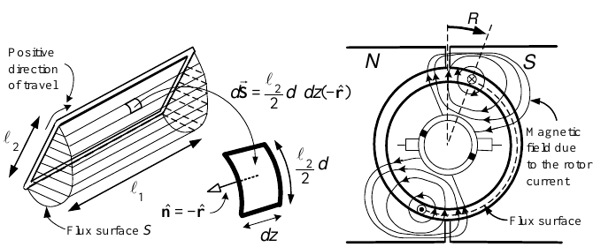
\[ \begin{aligned} \psi(i) &=\int_{S}\vec{\mathbf B}\cdot d\vec{\mathbf S}\\ &=i\int_{0}^{\ell_{1}}\int_{\theta_{R}}^{\theta_{R}+\pi} K(r_{R},\theta-\theta_{R})r_{R}\,d\theta\,dz\\ &=Li. \end{aligned} \]

If \(-d\psi/dt=-L\,di/dt>0\), the induced emf drives current into the page on side \(a\) and out of the page on side \(a'\).
\(-d\psi/dt\) has the same sign convention as \(V_{S}\).

Dynamic Equations of the DC Motor

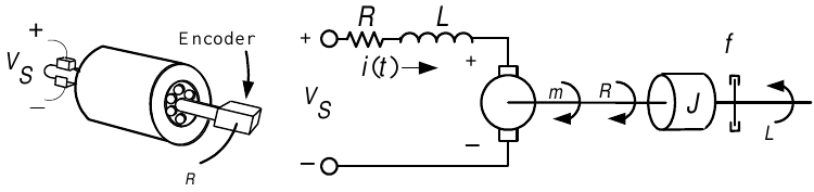
Electrical equation: \[ V_{S}-K_{b}\omega_{R}-L\frac{di}{dt}=Ri, \qquad L\frac{di}{dt}=-Ri-K_{b}\omega_{R}+V_{S}. \]

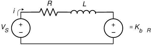
Mechanical equation: \[ K_{T}i-\tau_{L}-f\omega_{R}=J\frac{d\omega_{R}}{dt}. \]

\(J\): rotor-assembly moment of inertia.
\(\tau_{L}\): load torque.
\(f\): viscous-friction coefficient.

Equations of the DC Motor

\[ \begin{aligned} L\frac{di}{dt} &= -Ri-K_{b}\omega_{R}+V_{S},\\[0.45em] J\frac{d\omega_{R}}{dt} &= K_{T}i-f\omega_{R}-\tau_{L},\\[0.45em] \frac{d\theta_{R}}{dt} &= \omega_{R}. \end{aligned} \]

Energy Conversion

From the source voltage, \[ V_{S}=Ri+L\frac{di}{dt}+\xi. \]

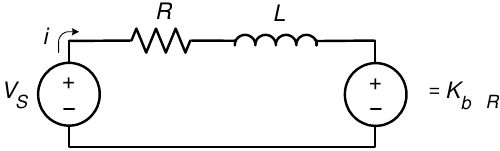
Multiplying by current gives \[ \begin{aligned} V_{S}i &=Ri^{2}+Li\frac{di}{dt}+iK_{b}\omega_{R}\\ &=Ri^{2}+\frac{d}{dt}\left(\frac{1}{2}Li^{2}\right) +\tau_{m}\omega_{R}. \end{aligned} \]

\(Ri^{2}\): heat loss.
\(d(\tfrac12Li^{2})/dt\): power stored in or recovered from the armature field.
\(\tau_{m}\omega_{R}\): mechanical power.

Optical Encoder

The encoder shown has 12 windows.
Digital circuitry detects each rising and falling pulse edge.
Twelve pulses produce 24 detectable edges per revolution.
Resolution: \(2\pi/24\) radians, or \(360^{\circ}/24=15^{\circ}\).
Counting the edges determines position to within \(15^{\circ}\).

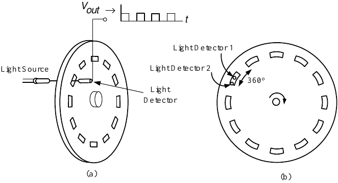
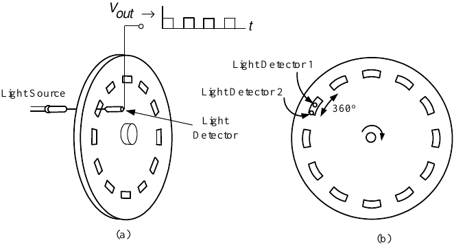
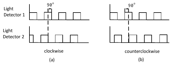
Optical Encoder Voltage Waveforms

Voltage waveforms from the encoder:

Quadrature Optical Encoder

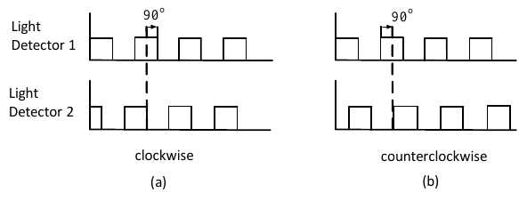
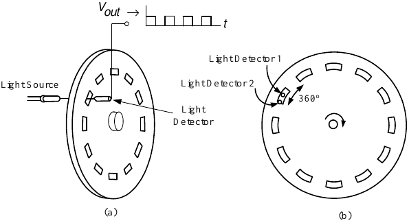
Window length equals the distance between adjacent windows.
The two light detectors are separated by half a window length.
One voltage-waveform period corresponds to the distance from one window’s beginning to the next.
Treating one period as \(360^{\circ}\) places the detectors \(90^{\circ}\) apart—in quadrature.

Optical Encoder Direction

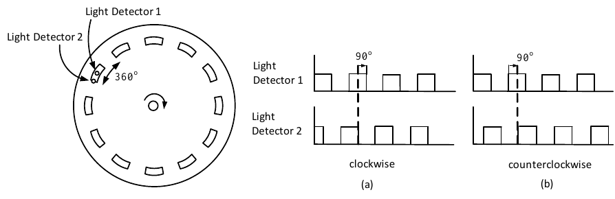
Clockwise rotation: detector 1 is \(90^{\circ}\) behind detector 2.

Counterclockwise rotation: detector 2 is \(90^{\circ}\) behind detector 1.

Electronic circuitry detects the relative phase to determine the direction.

Encoder Resolution

With \(N_{w}\) windows, \(2N_{w}\) rising and falling edges per revolution give resolution \[\frac{2\pi}{2N_{w}}\text{ radians}.\]
Counting both detector outputs gives \(4N_{w}\) equally spaced edges and resolution \[\frac{2\pi}{4N_{w}}\text{ radians}.\]
For \(N_{w}=500\), resolution is \(2\pi/2000\) radians, or \(0.18^{\circ}\).

Encoder Model

Let \(N_{enc}\) be the number of rising and falling edges from both detectors per revolution, and let \(N(t)\) be the encoder count at time \(t\).

\[ \theta_{m}(t)=\frac{2\pi}{N_{enc}}N(t)\quad\text{radians}. \]

Backward-difference speed estimate

\[ \omega_{bd}(kT) \triangleq\frac{2\pi}{N_{enc}} \left(\frac{N(kT)-N(kT-T)}{T}\right), \]

where \(T\) is the sampling interval.

Error in Backward-Difference Speed Estimation

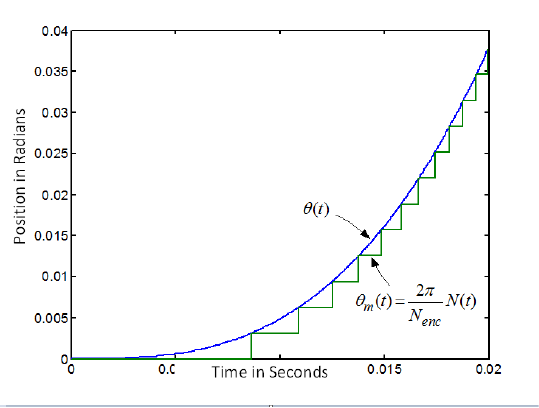
If \(\theta(kT)\) is the true position in radians, then \[ \theta(kT)=\frac{2\pi}{N_{enc}}N(kT) +\frac{2\pi}{N_{enc}}e(kT), \] where \(e(kT)\) is the fractional count that the encoder cannot sense.

Error in Backward-Difference Speed Estimation

The fractional count satisfies \(0\leq e(kT)<1\).

\[ \omega(kT) =\frac{2\pi}{N_{enc}} \left(\frac{N(kT)-N(kT-T)}{T}\right) +\frac{2\pi}{N_{enc}} \left(\frac{e(kT)-e(kT-T)}{T}\right). \]

Because \(\lvert e(kT)-e(kT-T)\rvert\leq1\), \[ \left\lvert\omega(kT)-\omega_{bd}(kT)\right\rvert \leq\frac{2\pi/N_{enc}}{T}. \]
Thus \[ \omega(kT)\approx\frac{2\pi}{N_{enc}} \left(\frac{N(kT)-N(kT-T)}{T}\right). \]
Choosing \(T\) trades encoder-resolution error against finite-difference accuracy.

The Physics of the DC Motor

Contents