Mass-Spring-Damper Systems

System Modeling and Control · Chapter 4

John N. Chiasson and Aykut C. Satici

Contents

• Mechanical Work

• Mass–Spring–Damper Systems

• Simulation

Mechanical Work

• A mass \(m\) moves along the \(x\)-axis with a force \(F\) acting on it.

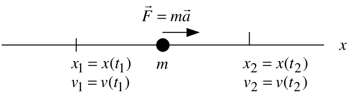
• \(x(t)\), \(v(t)=\dfrac{dx(t)}{dt}\), and \(a(t)=\dfrac{d^2x(t)}{dt^2}\) denote position, velocity, and acceleration.

• By Newton’s law, \[F=ma=m\frac{dv}{dt}=m\frac{d^2x}{dt^2}.\]

• The work \(W\) done on \(m\) by \(F\) from \(x_1\) to \(x_2\) is \[W\triangleq\int_{x_1}^{x_2}F(x)\,dx.\]

• Define \(x_1=x(t_1)\), \(v_1=v(t_1)\), \(x_2=x(t_2)\), and \(v_2=v(t_2)\). Then \[W=\int_{x_1}^{x_2}F(x)\,dx =\int_{t_1}^{t_2}\underbrace{m\frac{dv}{dt}}_{F}\underbrace{v\,dt}_{dx}.\]

Work and Kinetic Energy

We have

\[\begin{aligned} W\triangleq\int_{x_1}^{x_2}F(x)\,dx &=\int_{t_1}^{t_2}m\frac{dv}{dt}v\,dt \\ &=\int_{t_1}^{t_2}\frac{d}{dt}\left(\frac{mv^2}{2}\right)dt \\ &=\left.\frac{mv^2}{2}\right|_{v_1}^{v_2} \\ &=\frac{1}{2}mv_2^2-\frac{1}{2}mv_1^2. \end{aligned}\]

• The kinetic energy (KE) of the mass is defined to be \(\dfrac{1}{2}mv^2\).

• The work done on \(m\) equals the change in its kinetic energy: \[\int_{x_1}^{x_2}F(x)\,dx =\frac{1}{2}mv_2^2-\frac{1}{2}mv_1^2.\]

Example Horizontal Mass–Spring–Damper System

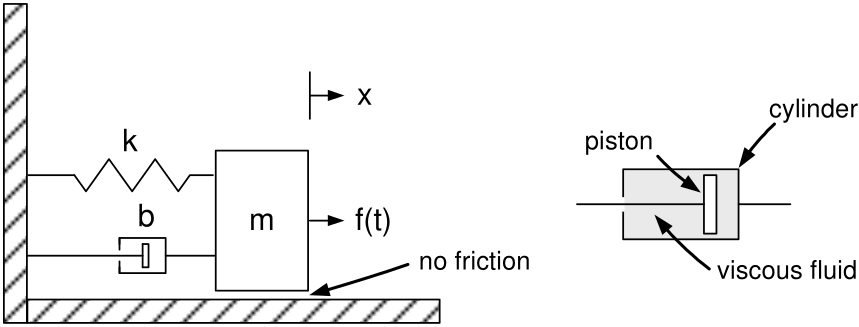
• If \(x=0\), the spring is neither compressed nor stretched—it is relaxed.

• The force on the mass \(m\) due to the spring is \(F_{mk}=-kx\).

  • If \(x>0\), the spring pulls \(m\) to the left.
  • If \(x<0\), the spring pushes \(m\) to the right.

• A damper consists of a piston encased in a sealed, fluid-filled cylinder. The piston’s motion is opposed by the viscous fluid.

• The force of the damper on \(m\) is \(F_{mb}=-b\dot{x}\).

  • If \(\dot{x}>0\), the fluid provides a resistive force in the \(-x\) direction.
  • If \(\dot{x}<0\), the fluid provides a resistive force in the \(+x\) direction.

Example Horizontal Mass–Spring–Damper System (continued)

\(f(t)\) denotes an external force:

\[m\frac{d^2x}{dt^2}=-kx-b\frac{dx}{dt}+f(t),\]

or

\[m\frac{d^2x}{dt^2}+b\frac{dx}{dt}+kx=f(t).\]

With zero initial conditions, the Laplace transform gives

\[(ms^2+bs+k)X(s)=F(s),\]

so

\[X(s)=\frac{1}{ms^2+bs+k}F(s).\]

With nonzero initial conditions,

\[X(s)= \underbrace{\frac{1}{ms^2+bs+k}}_{\text{transfer function}} \underbrace{F(s)}_{\text{input}} +\underbrace{\frac{mx(0)s+bx(0)+m\dot{x}(0)}{ms^2+bs+k}}_{\text{initial-condition response}}.\]

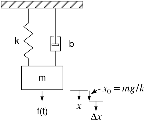
Example: Vertical Mass–Spring–Damper System

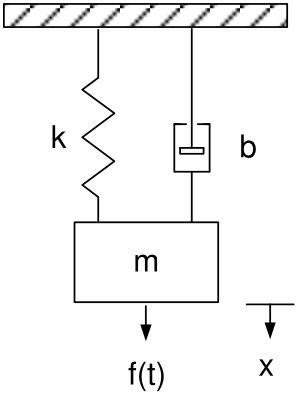
Equations of motion:

\[m\frac{d^2x}{dt^2}=-kx-b\frac{dx}{dt}+mg+f(t),\]

or

\[m\frac{d^2x}{dt^2}+b\frac{dx}{dt}+kx=mg+f(t).\]

At \(x=0\), the spring is relaxed. With zero initial conditions,

\[(ms^2+bs+k)X(s)=F(s)+\frac{mg}{s},\]

so

\[X(s)=\frac{1}{ms^2+bs+k}\left(F(s)+\frac{mg}{s}\right).\]

Example: Vertical Mass–Spring–Damper System (continued)

With \(f(t)\equiv0\),

\[m\frac{d^2x}{dt^2}+b\frac{dx}{dt}+kx=mg.\]

• Equilibrium means the mass \(m\) is at rest: \(\dot{x}=\ddot{x}\equiv0\).

• At equilibrium, \(kx_0=mg\), so \(x_0=mg/k\). With \(\Delta x=x-x_0\),

\[\begin{aligned} m\frac{d^2}{dt^2}(\Delta x+x_0) +b\frac{d}{dt}(\Delta x+x_0) +k(\Delta x+x_0)&=mg+f(t),\\ m\frac{d^2\Delta x}{dt^2} +b\frac{d\Delta x}{dt} +k\Delta x +\underbrace{m\frac{d^2x_0}{dt^2}+b\frac{dx_0}{dt}}_{0} +\underbrace{kx_0}_{mg}&=mg+f(t),\\ m\frac{d^2\Delta x}{dt^2} +b\frac{d\Delta x}{dt} +k\Delta x&=f(t). \end{aligned}\]

Example: Mass–Spring–Damper System with Two Masses

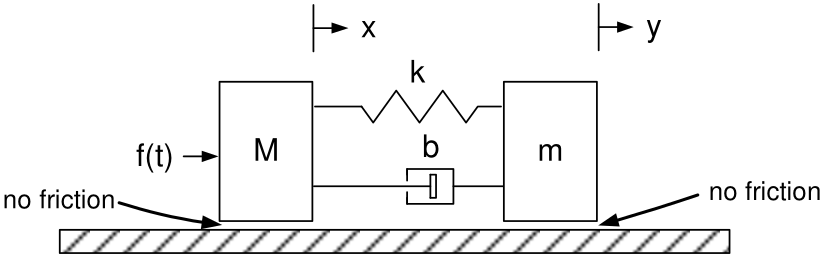
• The input is \(f(t)\) and the output is \(y(t)\). The references \(x\) and \(y\) locate \(M\) and \(m\), respectively.

• If \(x=y\), the spring is relaxed.

• Spring forces: \(F_{mk}=-k(y-x)\) and \(F_{Mk}=+k(y-x)\).

  • If \(y-x>0\), the spring pulls \(m\) in the \(-y\) direction and \(M\) in the \(+x\) direction.

• Damper forces: \(F_{mb}=-b(\dot{y}-\dot{x})\) and \(F_{Mb}=+b(\dot{y}-\dot{x})\).

  • If \(\dot{y}-\dot{x}>0\), the cylinder \(m\) moves right faster than the piston \(M\).
  • The piston produces a resistive force on the cylinder, while the cylinder drags the piston to the right.

Example: Mass–Spring–Damper System with Two Masses (continued)

Equations of motion:

\[\begin{aligned} m\frac{d^2y}{dt^2} &=\underbrace{-k(y-x)}_{F_{mk}}-\underbrace{b(\dot{y}-\dot{x})}_{F_{mb}},\\ M\frac{d^2x}{dt^2} &=\underbrace{k(y-x)}_{F_{Mk}}+\underbrace{b(\dot{y}-\dot{x})}_{F_{Mb}}+f(t). \end{aligned}\]

Equivalently,

\[\begin{aligned} m\frac{d^2y}{dt^2}+b\dot{y}+ky&=kx+b\dot{x},\\ M\frac{d^2x}{dt^2}+b\dot{x}+kx&=ky+b\dot{y}+f(t). \end{aligned}\]

With zero initial conditions, the Laplace transforms are

\[\begin{aligned} (ms^2+bs+k)Y(s)&=(bs+k)X(s),\\ (Ms^2+bs+k)X(s)&=(bs+k)Y(s)+F(s). \end{aligned}\]

Example: Mass–Spring–Damper System with Two Masses (continued)

From the previous slide,

\[\begin{aligned} (ms^2+bs+k)Y(s)&=(bs+k)X(s),\\ (Ms^2+bs+k)X(s)&=(bs+k)Y(s)+F(s). \end{aligned}\]

Eliminate \(X(s)\) to solve for \(Y(s)\):

\[\begin{aligned} (Ms^2+bs+k)\frac{ms^2+bs+k}{bs+k}Y(s)&=(bs+k)Y(s)+F(s),\\ (Ms^2+bs+k)(ms^2+bs+k)Y(s)&=(bs+k)^2Y(s)+(bs+k)F(s). \end{aligned}\]

Then

\[\begin{aligned} Y(s)&=\frac{bs+k}{(Ms^2+bs+k)(ms^2+bs+k)-(bs+k)^2}F(s)\\ &=\underbrace{\frac{bs+k}{Mms^4+(Mb+mb)s^3+(Mk+mk)s^2}}_{\text{transfer function }G(s)}F(s). \end{aligned}\]

• \(G(s)\) is unstable because it has two poles at \(s=0\).

Example Spring–Mass–Damper System with a Massless Point

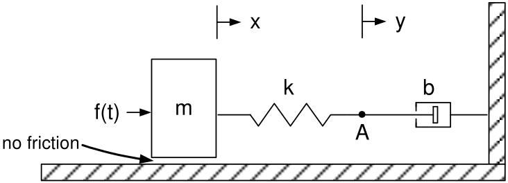
• Point \(A\) is the massless connection point of the spring and piston; \(y(t)\) locates it.

• The input is \(f(t)\) and the output is \(y(t)\).

• First let point \(A\) have a small mass \(m_A\); later let \(m_A\to0\).

\[\begin{aligned} m\frac{d^2x}{dt^2}&=k(y-x)+f(t),\\ m_A\frac{d^2y}{dt^2}&=-k(y-x)-b\frac{dy}{dt}. \end{aligned}\]

Equivalently,

\[\begin{aligned} m\frac{d^2x}{dt^2}+kx&=ky+f(t),\\ m_A\frac{d^2y}{dt^2}+b\frac{dy}{dt}+ky&=kx. \end{aligned}\]

Example Spring–Mass–Damper System with a Massless Point (continued)

From the previous slide,

\[\begin{aligned} m\frac{d^2x}{dt^2}+kx&=ky+f(t),\\ m_A\frac{d^2y}{dt^2}+b\frac{dy}{dt}+ky&=kx. \end{aligned}\]

Let \(m_A\to0\) and take Laplace transforms with zero initial conditions:

\[\begin{aligned} (ms^2+k)X(s)&=kY(s)+F(s),\\ (bs+k)Y(s)&=kX(s). \end{aligned}\]

Eliminating \(X(s)\) gives

\[(ms^2+k)(bs+k)Y(s)=k^2Y(s)+kF(s),\]

and therefore

\[Y(s)=\frac{k}{(ms^2+k)(bs+k)-k^2}F(s) =\underbrace{\frac{k}{bms^3+kms^2+bks}}_{\text{transfer function }G(s)}F(s).\]

\(G(s)\) is unstable because it has a pole at \(s=0\).

Example: Position Input and Massless Point

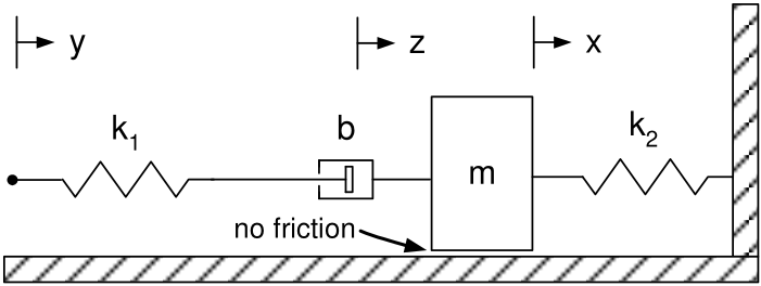
• The input is the position \(y\); the output is the position \(x\).

• No mass is shown on the right side of the spring.

  • Let \(m_p\) denote the mass of the piston to which the spring is attached.
  • Later, let \(m_p\to0\).
  • \(z\) denotes the piston position.

• If \(y=z\), spring \(k_1\) is relaxed; if \(x=0\), spring \(k_2\) is relaxed.

• The relative velocity between the piston and cylinder is \(\dot{z}-\dot{x}\).

Equations of motion:

\[\begin{aligned} m\ddot{x}&=-k_2x+b(\dot{z}-\dot{x}),\\ m_p\ddot{z}&=-b(\dot{z}-\dot{x})-k_1(z-y). \end{aligned}\]

Example: Position Input and Massless Point (continued)

\[\begin{aligned} m\ddot{x}&=-k_2x+b(\dot{z}-\dot{x}),\\ m_p\ddot{z}&=-b(\dot{z}-\dot{x})-k_1(z-y). \end{aligned}\]

Rearrange and take Laplace transforms with zero initial conditions:

\[\begin{aligned} m\ddot{x}+k_2x+b\dot{x}&=b\dot{z}, & (ms^2+bs+k_2)X(s)&=bsZ(s),\\ m_p\ddot{z}+b\dot{z}+k_1z&=b\dot{x}+k_1y, & (m_ps^2+bs+k_1)Z(s)&=bsX(s)+k_1Y(s). \end{aligned}\]

Eliminate \(Z(s)\):

\[(m_ps^2+bs+k_1)(ms^2+bs+k_2)X(s) =b^2s^2X(s)+k_1bsY(s).\]

Let \(m_p=0\):

\[\begin{aligned} X(s) &=\frac{k_1bs}{(bs+k_1)(ms^2+bs+k_2)-b^2s^2}Y(s)\\ &=\underbrace{\frac{k_1bs}{bms^3+mk_1s^2+(bk_1+bk_2)s+k_1k_2}}_{\text{transfer function}}Y(s). \end{aligned}\]

Simulation

First-Order System

\[\frac{dx}{dt}=-ax+bu,\qquad x(0)=x_0.\]

Convert to discrete time. Let \(x(kT)\) and \(u(kT)\) denote the values of \(x(t)\) and \(u(t)\) at time \(kT\).

Approximate \(dx/dt\) at time \((k+1)T\) by

\[\left.\frac{dx}{dt}\right|_{t=(k+1)T} =\frac{x((k+1)T)-x(kT)}{T}.\]

The discrete-time model is

\[\frac{x((k+1)T)-x(kT)}{T}=-ax(kT)+bu(kT), \qquad x(0)=x_0.\]

Rearranging,

\[x((k+1)T)=(1-aT)x(kT)+Tbu(kT), \qquad x(0)=x_0.\]

Discrete-Time Model

A digital computer simulates the discrete-time model

\[x((k+1)T)=(1-aT)x(kT)+Tbu(kT), \qquad x(0)=x_0.\]

For example, let \(x_0=1\) and \(u(t)=\cos(t)\). Then

\[\begin{aligned} x(T)&=(1-aT)x(0)+Tb\cos(0),\\ x(2T)&=(1-aT)x(T)+Tb\cos(T),\\ x(3T)&=(1-aT)x(2T)+Tb\cos(2T),\\ &\ \vdots \end{aligned}\]

That is, digital computers implement recursive algorithms.

Simulink Diagram

\[\frac{dx}{dt}=-ax+bu,\qquad x(0)=x_0.\]

Let \(u\) be a unit-step input. A Simulink diagram for this system is

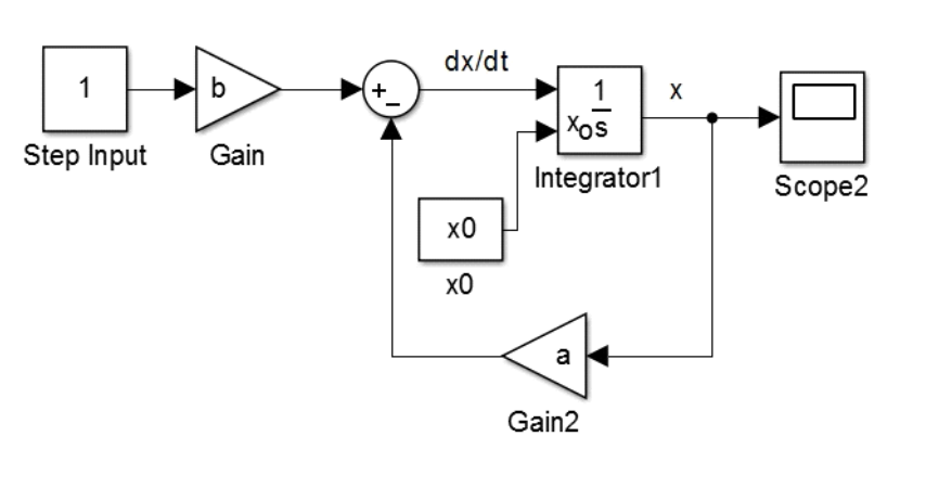
Simulink converts the block diagram to the discrete-time form

\[x((k+1)T)=(1-aT)x(kT)+Tbu(kT), \qquad x(0)=x_0.\]

Simulink uses \(1/s\) to denote the integration block.

Simulink Diagram (continued)

With zero initial conditions, we can represent

\[\frac{dx}{dt}=-ax+bu\]

by

\[X(s)=\frac{b}{s+a}U(s).\]

The Simulink block diagram is

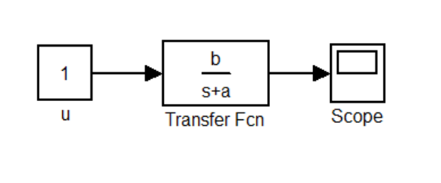
• Simulink then converts this to \[x((k+1)T)=(1-aT)x(kT)+Tbu(kT).\]

• When using a transfer-function block, Simulink assumes zero initial conditions.

• \(u\) is a unit-step input, so a “1” is inside the constant block.

  • \(u(kT)=1\) for \(k=0,1,2,\ldots\)
  • Do not put \(1/s\) in this block.

Example Simulation of \(m\dfrac{d^2x}{dt^2}=-kx-b\dfrac{dx}{dt}+f(t)\)

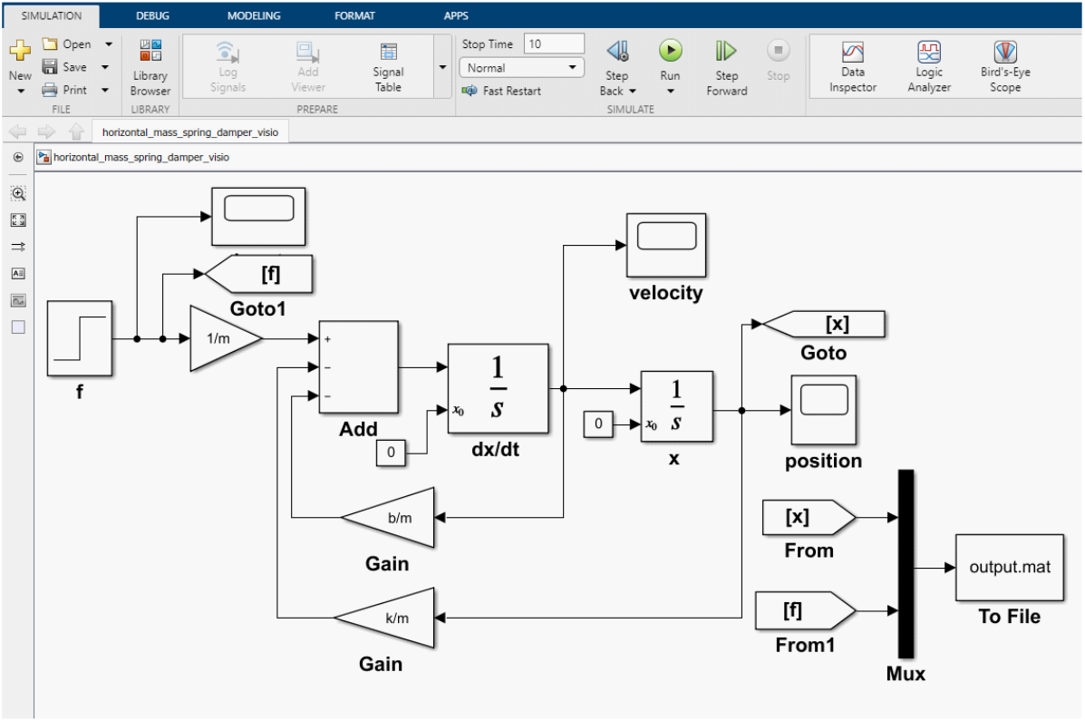
• SIMULATION is selected at the upper left of the Simulink file.

• Click MODELING, then click Model Settings (the gear icon).

• This opens the Configuration Parameters dialog box.

Example Simulation of \(m\dfrac{d^2x}{dt^2}=-kx-b\dfrac{dx}{dt}+f(t)\) (continued)

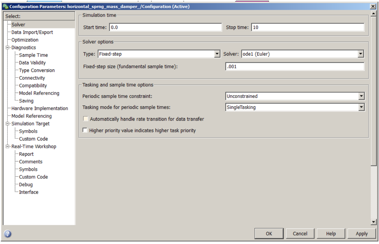
Dialog box for the Configuration Parameters.

Example Simulation of \(m\dfrac{d^2x}{dt^2}=-kx-b\dfrac{dx}{dt}+f(t)\) (continued)

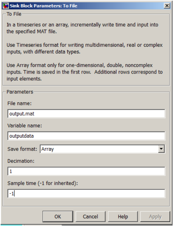
• The data is stored in a MATLAB data file called output.mat.

• Double-click the “To File” block to open it.

  • The data in this file is called outputdata.
  • It is an array (matrix) of three rows.
  • The first row is time \(t\), the second is position \(x\), and the third is the input \(f\).