Does the Turbine Need to Probe?

Aerodynamic torque is reconstructible for free, and the wind is already sweeping the curve

Aykut C. Satici

Robot Control Lab · Systems Engineering · UT Dallas

What probing costs

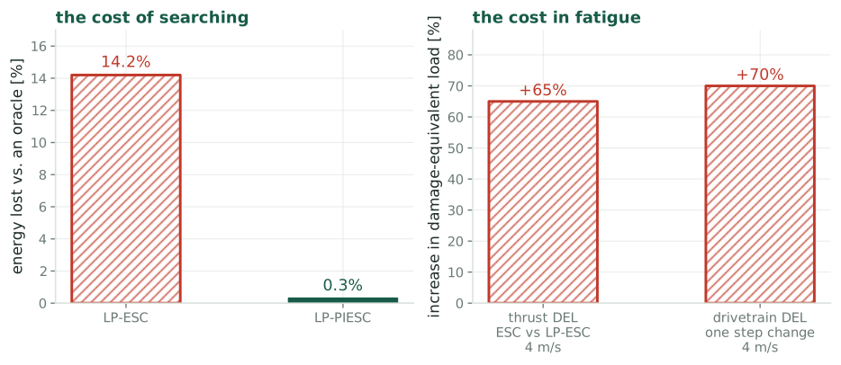
Searching is not free. It costs energy while you search, and it costs fatigue whether or not you find anything. Every design choice in this line is a trade against those two numbers.

The energy figure is measured against a controller that already knows the optimal gain, so it is the pure cost of not knowing. LP-PIESC brings it to 0.3 per cent, which is what makes the approach deployable at all.

The load figures are worth keeping in view because they do not shrink with better estimation. They are the price of moving the machine.

What comes for free

The rotor equation is \(I\dot\Omega = T_{\text{aero}} - \tau_{\text{gen}}\), and every term on the right is known. \(\tau_{\text{gen}}\) is commanded, \(\Omega\) is measured by an encoder, \(I\) is a design constant. So

\[T_{\text{aero}}(t) \;=\; I\dot\Omega(t) + \tau_{\text{gen}}(t)\]

is exactly reconstructible with no anemometer, and it satisfies

\[T_{\text{aero}} \;=\; \tfrac12\rho\pi R^3 V^2\, C_Q\!\left(\frac{R\Omega}{V}\right)\]

Two unknowns: the wind path \(V(t)\) and the function \(C_Q(\cdot)\). The question is whether the record of \((\Omega,\,T_{\text{aero}})\) determines them.

Note what this quietly resolves. The generator-versus-aerodynamic-power problem, the one the 2024 ACC paper is about, disappears here: the inertial term is not a contaminant to be filtered out, it is the signal being used.

The wind is already doing the experiment

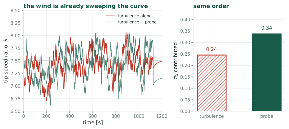
Turbulence sweeps \(\lambda\) with \(\sigma_\lambda \approx 0.24\), against the probe’s \(0.34\). Same order. The dither is not supplying excitation the wind lacks. It is supplying excitation the controller knows about.

The estimate is the fraction of turbulence energy above the rotor’s own pole, which is what the rotor cannot follow and so passes straight into lambda. At ten per cent intensity and a pole near 0.18 radians per second, roughly a ninth of the variance gets through.

Order of magnitude, not a measurement, and it does not need to be tight to make the point: the machine is swept across its own curve all day, and the fatigue cost of that sweep is being paid whether or not anyone uses it.

Exactly one blind direction

Substitute \(\tilde V = cV\) and ask which curve explains the same data:

\[\tilde C_Q(x) = \frac{C_Q(cx)}{c^2} \;\;\Longrightarrow\;\; \tilde C_P(x) = \frac{C_P(cx)}{c^3} \;\;\Longrightarrow\;\; \tilde\lambda^\star = \frac{\lambda^\star}{c}\]

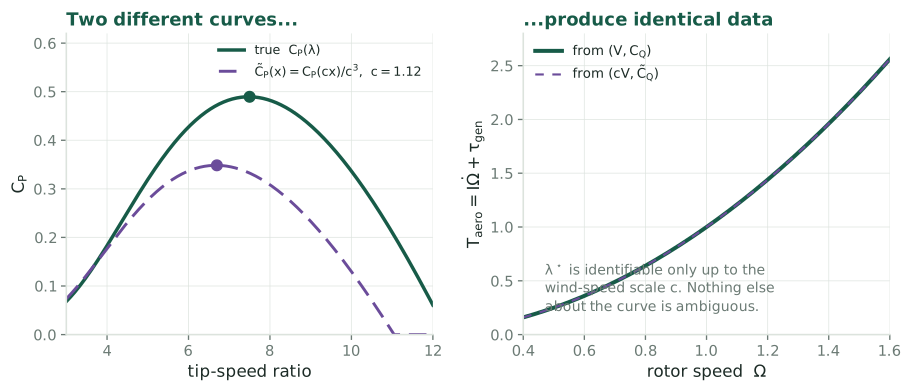
One unidentifiable direction, an overall scaling of the wind, mapping straight onto a scaling of \(\lambda^\star\). Everything else about the curve is determined.

And one thing that does not matter

Air density enters as a prefactor, so an error in \(\rho\) scales \(C_P\) uniformly:

\[\tilde C_P(x) = \frac{C_P(x)}{d} \;\;\Longrightarrow\;\; \tilde\lambda^\star = \lambda^\star\]

Wind speed scale

Moves the estimated peak. Must be pinned.

Air density

Does not move the peak. Can be left unknown.

Useful, because density is the quantity that varies with temperature and altitude and is usually estimated badly. It turns out not to matter for locating \(\lambda^\star\).

What breaks the degeneracy

What you do not need

A fast rotor-effective wind estimate. Those are reconstructed through a presumed \(C_P\) surface, which makes the whole exercise circular.

What you do need

One slowly updated absolute wind scale, to pin the constant \(c\). A met mast, a nacelle lidar, or a long-run SCADA average.

A slow reference is also far harder to contaminate with the control parameter. The induction response that makes nacelle estimates circular is fast, and it does not reach a monthly average.

This is the part that makes the idea practical rather than merely elegant. The usual objection is that you cannot separate the wind from the curve, and that is true, but it is true in exactly one direction, and that direction is the one a site already has an instrument for.

The test

Take an existing simulation run with the dither switched off. Reconstruct \(T_{\text{aero}} = I\dot\Omega + \tau_{\text{gen}}\), fit a parametrized \(C_Q(\cdot)\) jointly with the wind path, pin the scale with the known mean wind, and compare the recovered peak against the simulator’s own answer.

What makes it cheap

No new runs. Every quantity needed is already logged in the existing output, and the dither-off case is the baseline condition.

What decides it

Whether the recovered \(\lambda^\star\) lands within the tolerance the erosion problem needs, which is about \(0.1\).

Risks, stated plainly

Prior art

This sits close to the wind-speed-estimator literature, which assumes \(C_P\) known and solves for \(V\). The joint version is what would be new, and that claim needs checking first.

Differentiation

\(T_{\text{aero}}\) needs \(\dot\Omega\), and differentiating a noisy encoder signal is where this could fail in practice rather than in principle.

Identifiability in practice

One blind direction in theory does not guarantee a well-conditioned fit. The degeneracy could be nearly degenerate in more directions than one.

Of the three questions this is the riskiest and the one with the largest payoff. It does not improve the probing trade-off. It removes it.

Does the turbine need to probe?

The dither exists because the excitation is unknown, not because excitation is lacking.

The claim

Aerodynamic torque is reconstructible with no wind sensor, turbulence supplies comparable excitation to the probe, and the joint estimation problem has exactly one blind direction, which a slow absolute reference pins.

If it holds

No dither. No fatigue cost of probing, no amplitude to choose, no frequency plan, and the bias-variance trade of the estimand question disappears with it.

Kumar & Rotea, Energies 2022 · Ciri, Leonardi & Rotea, Wind Energy 2019 · Mulders, Gallo & Rotea, ACC 2024 · Soltani et al. on rotor-effective wind estimation

One of three: see also the estimand and the speed limit.